library(tidyverse)

tech_october <- read_csv("https://bcdanl.github.io/data/tech_stocks_2025_10.csv") |>
  mutate(Date = as.Date(Date)) |>
filter(Ticker %in% c("MSFT", "META"))Classwork 16
Time Trends and a Short Data Story
NoteNote
Complete the questions and submit your responses on the corresponding Brightspace page.
Complete the code in an R script and keep your brief written interpretations with it. This page contains its own setup and data definitions; no earlier classwork is required.
Setup and data
The course file contains daily stock-trading records from October 1–30, 2025. Use Microsoft and Meta to study daily trading volume, the number of shares traded during a day. The supplied code converts Date into calendar dates and keeps these two companies.
| Variable | Meaning |
|---|---|
Date |
Trading day |
Ticker |
Company identifier: MSFT = Microsoft, META = Meta |
Volume |
Number of shares traded during that trading day |
Each row represents one company’s trading record on one trading day. There are 22 observed trading days per company. Volume counts shares traded, not distinct traders or dollars. These are historical records, not current trading activity.
Filling-in-the-blank: 1. Trading activity over time
Complete the code to plot Volume against Date, with a separate line and color for each company.
ggplot(data = tech_october,
       mapping = aes(x = ____,
                     y = ____,
                     color = ____)) +
  ____()
What does a point on either line represent, and what are the vertical-axis units? Explain why connecting all rows as one line would misrepresent the data.
Interpretation: 2. Separate panels, shared scale
Use this supplied version to inspect the two histories separately. group = Ticker tells ggplot which observations belong together, even though both lines use one chosen color.
ggplot(data = tech_october,
       mapping = aes(x = Date,
                     y = Volume,
                     group = Ticker)) +
  geom_line(color = "#0072B2") +
  facet_wrap(~ Ticker) +
  labs(x = "Trading date",
       y = "Daily trading volume (shares)")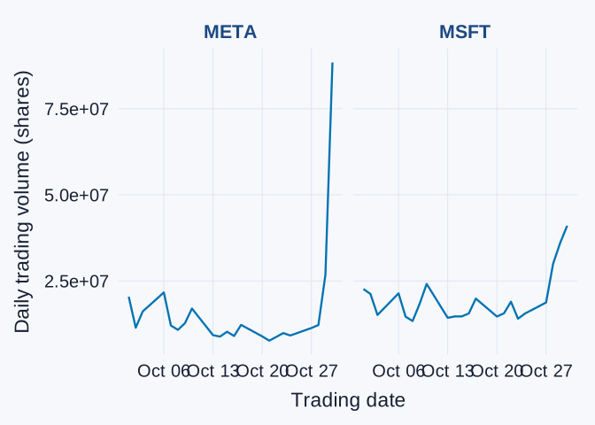
Compare the companies’ trading activity near the end of the interval. Which shows the larger late-month spike? Why are shared vertical-axis scales useful for this comparison? Explain why greater trading volume does not, by itself, establish a higher share price or a better investment return.
Interpretation: 3. Evidence for an audience
Choose one graph from this page and write a short paragraph for someone who has not seen the dataset:
- State a question about trading activity and identify what the observations represent.
- Describe a finding supported by the graph.
- Explain one limitation or piece of information you would want before explaining the changes in trading activity.
For a project draft, add an understandable title, axis labels with units, and a source. You may adapt a labs() example from the slides. Clear labeling matters for the project, but there is no requirement to memorize the function’s syntax.