library(tidyverse)
library(ggthemes)

flights <- nycflights13::flights
destination_flights <- flights |>
  filter(month == 1 | month == 7,
dest == "BOS" | dest == "LAX" | dest == "ORD")Classwork 13
Distribution of a Categorical Variable Across Groups
NoteNote
Complete the questions and submit your responses on the corresponding Brightspace page.
Fill each ____ with the appropriate variable, function, or value. Keep your completed code and brief interpretations together in an R script. This page has its own setup; no earlier classwork is required.
Setup and data
destination_flights contains 8,124 historical flight records from January and July 2013 with Boston, Los Angeles, or Chicago O’Hare as the destination. It includes all airlines and all three NYC-area departure airports in the data. Some records have no actual departure time, so these are flight-record counts rather than counts of completed trips. They are not passenger counts. Every comparison below is limited to these three destinations and two months.
| Variable | Meaning |
|---|---|
dest |
Destination airport: BOS = Boston Logan, LAX = Los Angeles International, ORD = Chicago O’Hare |
month |
1 = January, 7 = July |
factor(month) treats January and July as two categories. To read the full variable descriptions in R, run ?nycflights13::flights.
Filling-in-the-blank: 1. Compare monthly totals with stacked bars
Complete the plot with one stacked bar for each month and a different color for each destination airport.
ggplot(data = destination_flights,
       mapping = aes(x = factor(____),
                     fill = ____)) +
  geom_bar() +
  scale_fill_colorblind()
Which month has more flight records to the three selected destinations combined? What does each colored segment count, and what does the full bar height count? Why is the legend useful?
TipExample answer
ggplot(data = destination_flights,
       mapping = aes(x = factor(month),
                     fill = dest)) +
  geom_bar() +
  scale_fill_colorblind()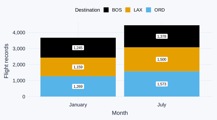
geom_bar() counts records and stacks the destination airports within each month. The height of an entire bar is that month’s total for the three selected destinations: 3,673 in January and 4,451 in July. July has 778 more flight records. Each colored section counts records for one destination in one month; the legend identifies the destination represented by each color.
Filling-in-the-blank: 2. Find each destination’s increase
Run this code. count(dest, month) creates a six-row table of flight-record counts for each destination and month.
destination_month_counts <- destination_flights |>
count(dest, month)| dest | month | n |
|---|---|---|
| BOS | 1 | 1245 |
| BOS | 7 | 1378 |
| LAX | 1 | 1159 |
| LAX | 7 | 1500 |
| ORD | 1 | 1269 |
| ORD | 7 | 1573 |
Complete a side-by-side bar chart so the January and July counts for each destination start from the same baseline.
ggplot(data = destination_flights,
       mapping = aes(x = dest,
                     fill = factor(month))) +
  geom_bar(position = "____") +
  scale_fill_colorblind()
Using the table, calculate July minus January for each destination. Which destination has the largest increase in flight-record count?
TipExample answer
ggplot(data = destination_flights,
       mapping = aes(x = dest,
                     fill = factor(month))) +
  geom_bar(position = "dodge") +
  scale_fill_colorblind()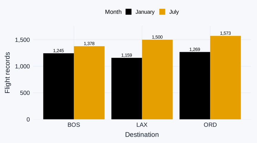
The side-by-side bars compare January and July counts for each destination. The table gives the exact values. Subtract January from July for each destination:
- BOS: 1,378 − 1,245 = 133 more records.
- LAX: 1,500 − 1,159 = 341 more records, the largest increase.
- ORD: 1,573 − 1,269 = 304 more records.
Filling-in-the-blank: 3. Read destination shares within a month
Complete a 100% stacked bar chart with one bar for January and one for July. Each bar shows the three selected destinations’ shares within that month.
ggplot(data = destination_flights,
       mapping = aes(x = factor(____),
                     fill = ____)) +
  geom_bar(position = "____") +
  scale_fill_colorblind()
For the LAX section of the July bar, give the numerator, denominator, and approximate percentage using the count table. Do the equal total heights of the two bars mean January and July had equal flight-record counts? Explain.
TipExample answer
ggplot(data = destination_flights,
       mapping = aes(x = factor(month),
                     fill = dest)) +
  geom_bar(position = "fill") +
  scale_fill_colorblind()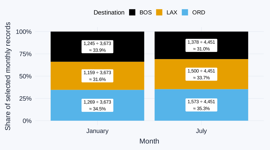
position = "fill" makes each month’s bar reach 1, or 100%. In the July bar, the LAX section uses 1,500 July LAX records out of 4,451 total July records to the three selected destinations:
LAX share of the selected July records: 1,500 ÷ 4,451 ≈ 33.7%.
The equal-height bars show shares, not equal record counts: January has 3,673 selected records and July has 4,451.
Filling-in-the-blank: 4. Reverse the grouping
Now place destination airports on the horizontal axis and use color for month. Complete another 100% stacked bar chart.
ggplot(data = destination_flights,
       mapping = aes(x = ____,
                     fill = factor(____))) +
  geom_bar(position = "____") +
  scale_fill_colorblind()
For the July section of the LAX bar, give the numerator, denominator, and approximate percentage. Why is this percentage different from the LAX July percentage in Question 3, even though both use the same LAX July records? Which plot answers “Among the three selected destinations, what share of July records were headed to LAX?” Which plot answers “Of all flight records with LAX as the destination in January and July combined, what percentage were from July?”
TipExample answer
ggplot(data = destination_flights,
       mapping = aes(x = dest,
                     fill = factor(month))) +
  geom_bar(position = "fill") +
  scale_fill_colorblind()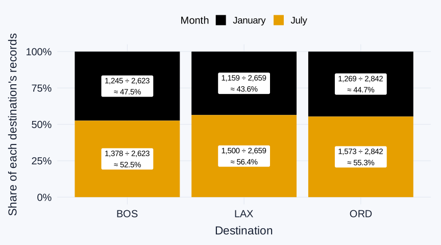
Now each destination’s bar reaches 1. For LAX, the July section is 1,500 July LAX records out of 2,659 LAX records across January and July:
July share of LAX’s January-and-July records: 1,500 ÷ (1,159 + 1,500) = 1,500 ÷ 2,659 ≈ 56.4%.
Questions 3 and 4 use the same flight records. Question 3 asks what share of July records to the three selected destinations were headed to LAX; Question 4 asks what share of LAX’s January-and-July records occurred in July. Changing the horizontal grouping changes the denominator. The 56.4% is a share within these two selected months, not LAX’s share for the whole year.