library(tidyverse)
library(ggthemes)Classwork 12
Distribution of a Categorical Variable
NoteNote
Complete the questions and submit your responses on the corresponding Brightspace page.
Complete the code in an R script and keep your brief written interpretations with it. This page contains its own setup and data definitions; no earlier classwork is required.
Setup and data
The built-in mpg data contains 234 vehicle model configurations from model years 1999 and 2008. Each row represents a configuration, not a vehicle sold or registered. The variable fl records fuel type: c = compressed natural gas (CNG), d = diesel, e = ethanol, p = premium gasoline, and r = regular gasoline. Dataset reference: ggplot2 · mpg.
Filling-in-the-blank: 1. Rows become counts
Count vehicle configurations by fuel type using horizontal bars.
ggplot(data = mpg,
       mapping = aes(y = ____,
                     fill = fl)) +
  ____() +
  scale_fill_colorblind()
What does the length of each bar represent? Why do these bars not tell us how many vehicles of each fuel type were sold or are on the road?
TipExample answer
ggplot(data = mpg,
       mapping = aes(y = fl,
                     fill = fl)) +
  geom_bar(show.legend = FALSE) +
  scale_fill_colorblind()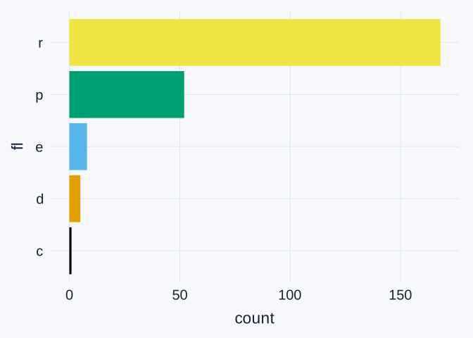
Each bar’s length is the number of configurations with that fuel type. For example, the r (regular gasoline) bar represents 168 rows of mpg. geom_bar() calculates these counts from the original rows; we do not supply a count column.
fill = fl gives the bars fuel-type colors. The axis labels identify the fuel codes, so show.legend = FALSE removes a duplicate legend.
These counts describe the configurations in this dataset. They do not count vehicles sold or registered, and the data do not establish how many vehicles of each fuel type are on the road. That would require sales or registration counts.
Filling-in-the-blank: 2. Counts already stored in a table
Run this supplied preparation code. count(fl) creates one row per fuel type and stores the number of configurations in a new column named n.
fuel_counts <- mpg |>
count(fl)| fl | n |
|---|---|
| c | 1 |
| d | 5 |
| e | 8 |
| p | 52 |
| r | 168 |
Plot those existing counts with geom_col().
ggplot(data = fuel_counts,
       mapping = aes(x = ____,
                     y = fl,
                     fill = fl)) +
  ____() +
  scale_fill_colorblind()
Explain why geom_col() suits fuel_counts, while geom_bar() suits the original mpg table.
TipExample answer
fuel_counts has five rows, one per fuel type. The n column already stores the number of configurations for each fuel type: c 1, d 5, e 8, p 52, and r 168.
ggplot(data = fuel_counts,
       mapping = aes(x = n,
                     y = fl,
                     fill = fl)) +
  geom_col(show.legend = FALSE) +
  scale_fill_colorblind()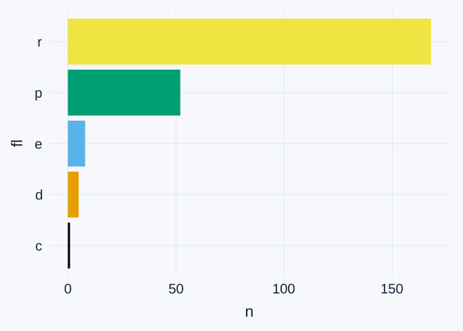
geom_col() draws bars using the values already stored in n: mapping x = n makes bar length equal to that count. In contrast, geom_bar() is appropriate for the original mpg rows because it counts those configurations for us.
Using geom_bar() with only y = fl on fuel_counts would count the rows in the summary table. Because there is only one row per fuel type, it would produce counts of one instead of the original configuration counts.
Interpretation: 3. A sorted comparison
Use this supplied version to sort fuel-type labels by count. fct_reorder(fl, n) orders the labels using n.
ggplot(data = fuel_counts,
       mapping = aes(x = n,
                     y = fct_reorder(fl, n),
                     fill = fl)) +
  geom_col() +
  scale_fill_colorblind()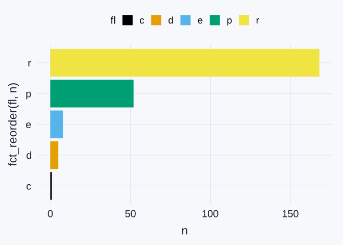
Which fuel type has the most configurations, and which has the fewest? Give their codes, full names, and counts. Does sorting change the label order compared with Question 2? Use the count table to explain.
TipExample answer
The largest count is r (regular gasoline), with 168 configurations. The smallest is c (compressed natural gas), with 1 configuration. The other counts are d (diesel) 5, e (ethanol) 8, and p (premium gasoline) 52.
Sorting does not visibly change the order here. The original fuel codes are already arranged c, d, e, p, r, and their counts increase in that same order: 1, 5, 8, 52, 168. fct_reorder(fl, n) still orders labels by count, but it produces the same order for this particular table. Neither plot measures sales or the number of vehicles on the road.
Interpretation: 4. Follow-up: when sorting changes the bar order
Now use another categorical variable in the same mpg data: drv identifies the drive type. The codes are 4 = four-wheel drive, f = front-wheel drive, and r = rear-wheel drive.
Run this preparation code and compare the two supplied plots.
drv_counts <- mpg |>
count(drv)| Drive type | Configurations |
|---|---|
| 4 | 103 |
| f | 106 |
| r | 25 |
Original category order
ggplot(data = drv_counts,
       mapping = aes(x = n,
                     y = drv,
                     fill = drv)) +
  geom_col(show.legend = FALSE) +
  scale_fill_colorblind()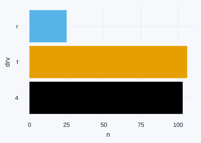
Sorted by count
ggplot(data = drv_counts,
       mapping = aes(x = n,
                     y = fct_reorder(drv, n),
                     fill = drv)) +
  geom_col(show.legend = FALSE) +
  scale_fill_colorblind()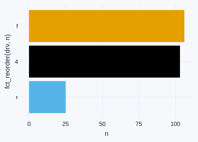
Explain why sorting changes the bar order here but did not change it for fuel type in Question 3. Does sorting change the counts or the color assigned to each drive type?
TipExample answer
The default plot reads r, f, 4 from top to bottom. After sorting by count, it reads f, 4, r from top to bottom. The counts are 106 front-wheel-drive configurations (f), 103 four-wheel-drive configurations (4), and 25 rear-wheel-drive configurations (r).
The default drive-code order does not match increasing counts, so fct_reorder(drv, n) moves the bars. In Question 3, the fuel codes c, d, e, p, r already had increasing counts (1, 5, 8, 52, 168), so sorting left their order unchanged.
Sorting changes the bars’ vertical positions, not their counts or lengths. Because both plots map fill = drv, each drive type also keeps the same color.