library(tidyverse)Classwork 11
Distribution of a Numeric Variable Across Groups
NoteNote
Complete the questions and submit your responses on the corresponding Brightspace page.
Complete the code in an R script and keep your brief written interpretations with it. This page contains its own setup and data definitions; no earlier classwork is required.
Setup and data
The built-in mpg data contains 234 vehicle model configurations from model years 1999 and 2008. Each row represents a configuration, not an individual driver or purchase.
| Variable | Meaning |
|---|---|
cty |
City fuel economy in miles per gallon; higher means farther per gallon |
drv |
Drive type: f = front-wheel, r = rear-wheel, 4 = four-wheel |
Dataset reference: ggplot2 · mpg.
Filling-in-the-blank: 1. Histograms in separate panels
Make a separate histogram for each drive type. Use a bin width of 2 mpg in every panel and keep the default shared axis scales.
ggplot(data = mpg,
       mapping = aes(x = cty)) +
  geom_histogram(binwidth = 2) +
  ____(~ ____)
Use facet_wrap() and drv in the blanks. Describe one difference in typical fuel economy or spread between two drive types.
TipExample answer
ggplot(data = mpg,
       mapping = aes(x = cty)) +
  geom_histogram(binwidth = 2) +
  facet_wrap(~ drv)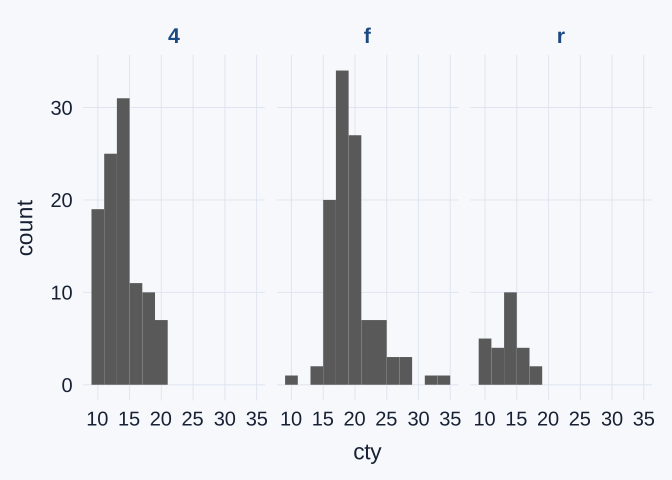
facet_wrap(~ drv) draws one panel per drive type, and binwidth = 2 is applied in every panel.
Typical fuel economy. Front-wheel-drive (f) vehicles are centered at higher city fuel economy than four-wheel-drive (4) vehicles. The tallest front-wheel bar is centered near 18 mpg, while the tallest four-wheel bar is centered near 14 mpg. The front-wheel distribution is shifted to the right.
Spread. The front-wheel panel is also more spread out. It has a long right tail, with a few configurations reaching 33–35 mpg, whereas the four-wheel configurations stay at or below about 21 mpg.
Interpretation: 2. Counts and group sizes
Refer to the faceted histograms from Question 1. Compare the same city-fuel-economy interval (bin) in two drive-type groups.
- A bar’s height is the number of vehicles in that interval; the corresponding proportion is that number divided by the total number of vehicles in that drive-type group.
Explain how different group totals can affect the comparison. You do not need to read exact counts or calculate exact proportions from the graph.
TipExample answer
The groups are not the same size: the data contain 103 four-wheel, 106 front-wheel, and only 25 rear-wheel configurations. A bar’s height is a count, so a group with more configurations tends to have taller bars even when its configurations are spread across the intervals in the same way.
| Interval | Group | Configurations in the bin | Group total | Proportion of the group |
|---|---|---|---|---|
| 13–15 mpg (centered on 14) | Four-wheel (4) |
31 | 103 | about 30% |
| 13–15 mpg (centered on 14) | Rear-wheel (r) |
10 | 25 | 40% |
In this interval, the four-wheel bar is about three times taller than the rear-wheel bar, yet the rear-wheel group has the larger proportion of its configurations there. The taller bar reflects the larger group, not a greater share of that group.
A taller bar therefore answers “which group has more vehicles in this interval?” To compare how likely a vehicle in each group is to fall in the interval, divide each count by its group total, or compare the shapes of the panels rather than the bar heights.
Filling-in-the-blank: 3. A boxplot comparison
Compare city fuel economy across drive types.
ggplot(data = mpg,
       mapping = aes(x = cty,
                     y = ____,
                     fill = ____)) +
  ____(show.legend = FALSE)
Describe a difference in typical fuel economy or spread.
TipExample answer
ggplot(data = mpg,
       mapping = aes(x = cty,
                     y = drv,
                     fill = drv)) +
  geom_boxplot(show.legend = FALSE)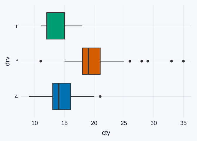
The vertical axis lists the drive types, and fill = drv colors each box by its group. Because drv is already labeled on the axis, show.legend = FALSE removes a redundant legend.
Typical fuel economy. The front-wheel median is about 19 mpg, compared with about 14 mpg for four-wheel. The front-wheel box (roughly 18–21 mpg) sits entirely to the right of the four-wheel box (roughly 13–16 mpg). The rear-wheel median is about 15 mpg, so its box overlaps heavily with the four-wheel box.
Spread. The three boxes are similar in width, with the middle 50% of each group spanning about 3 mpg. The front-wheel group stands out for its many individual points at high values, from 26 to 35 mpg, which the boxplot flags as unusually high for that group.
Interpretation: 4. Choose a useful comparison
The histogram shows detailed distribution shape; the boxplot provides a compact summary. Which graph better supports the comparison you described, and why?
TipExample answer
For the comparison of typical fuel economy, the boxplot is the better choice. The three medians (about 19, 14, and 15 mpg) and boxes sit side by side on one shared axis, so the front-wheel advantage over four-wheel is visible in a single glance. Because the boxplot summarizes each group by its quartiles, the very different group sizes (25 to 106 configurations) do not distort the comparison the way they affect bar heights in the faceted histograms.
The histograms are the better choice when the question is about shape: where the main peak is, how long the right tail of front-wheel vehicles runs, or how many configurations each group contains. The boxplot hides all of that. It does not show group sizes, and it cannot distinguish one broad peak from two separate peaks.
A good answer matches the graph to the comparison: use the boxplot for medians and spread, and the histogram for the full distribution shape.