Classwork 10

Distribution of a Numeric Variable

Author

Byeong-Hak Choe

Published

October 21, 2026

Note

Complete the questions and submit your responses on the corresponding Brightspace page.

Fill each ____ with the appropriate variable, function, argument, or value, then run your completed code in an R script. Keep your code and brief written interpretations together. This page contains everything you need to start; no earlier classwork is required.

Setup and data

library(tidyverse)

The built-in mpg data contains 234 vehicle model configurations from model years 1999 and 2008. Each row represents a configuration, not an individual driver or purchase. The variable cty records city fuel economy in miles per gallon: higher values mean a vehicle travels farther using one gallon of fuel. Dataset reference: ggplot2 · mpg.

Filling-in-the-blank: 1. Make two histograms

Make a histogram of city fuel economy with a bin width of 1 mpg. Then make a second version with a bin width of 5 mpg.

ggplot(data = mpg,
       mapping = aes(x = cty)) +
  geom_____(____)

ggplot(data = ____,
       mapping = aes(x = ____)) +
  ____(____)

Example answer

ggplot(data = mpg,
       mapping = aes(x = cty)) +
  geom_histogram(binwidth = 1)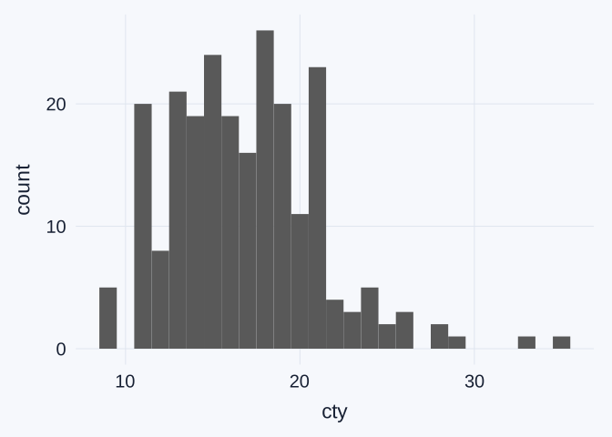

ggplot(data = mpg,
       mapping = aes(x = cty)) +
  geom_histogram(binwidth = 5)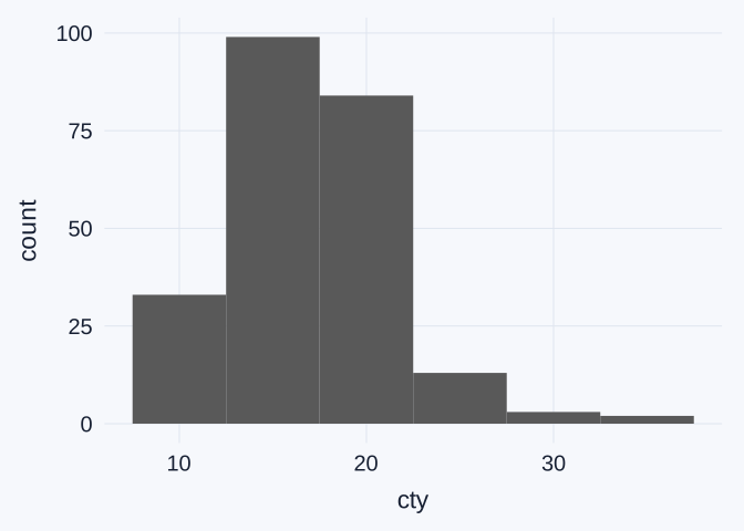

The first plot groups city fuel-economy values into intervals 1 mpg wide. The second uses intervals 5 mpg wide. Both display the same 234 configurations; changing the bin width changes how values are grouped, not the observations themselves.

Interpretation: 2. Read the plot instructions and axes

Identify the data, the variable mapped to x, and the geometric object used in your first plot (name its geom_*() function). What does its vertical axis count? Explain why no variable is mapped to y aesthetic: what does ggplot calculate from the observations?

Example answer

Part	Meaning in the first plot
`data = mpg`	Use the rows and columns of the `mpg` data frame.
`mapping = aes(x = cty)`	Place city fuel economy on the horizontal axis.
`geom_histogram(binwidth = 1)`	Group the values into 1-mpg intervals and draw bars showing their counts.

The geometric object is a set of histogram bars, drawn by geom_histogram().

The vertical axis counts configurations in each interval. It does not show fuel economy, sales, or the number of drivers. No variable is mapped to y because geom_histogram() calculates the counts from the cty observations.

For example, the 1-mpg histogram has 26 configurations in the bar centered on 18 mpg. With integer-valued cty, that bar counts configurations recorded as 18 mpg.

Interpretation: 3. Compare the bin widths

Describe one detail that the narrower bins show more clearly, or one pattern that the wider bins make easier to see.

Example answer

The 1-mpg bins reveal local bumps and gaps, such as an empty bin around 10 mpg and several small bars above 25 mpg. The 5-mpg bins make the broad pattern easier to see: most configurations are concentrated in the middle of the observed values, with relatively few at the high end.

In the 5-mpg version, the two tallest adjacent bins span approximately 12.5–22.5 mpg and together contain 183 of the 234 configurations. Calling this a common range is more appropriate than trying to read an exact median from the histogram. A histogram groups observations, so its bars do not identify the exact middle observation.

Interpretation: 4. Describe the peaks

Are bar heights roughly uniform, or do you see one clear peak (unimodal) or two clear peaks (bimodal)? Does changing the bin width change your description? Small bumps alone need not indicate separate groups.

Example answer

The bars are not roughly uniform. With 5-mpg bins, there is one broad main concentration, so roughly unimodal is a reasonable description. The 1-mpg version looks much bumpier, with several local high bars, rather than presenting two clearly separated main peaks.

The narrower bins do not provide strong evidence for calling this distribution bimodal. A small bump can result from the bin width and the integer-valued measurements. Changing the bin width can change the apparent number of peaks, so a good answer identifies which version it describes.

Interpretation: 5. Describe the tails

Is the longer tail toward smaller values (left-skewed) or larger values (right-skewed), or are the tails roughly balanced? Identify the tail from the values along the horizontal axis, rather than from the side with the tallest bars.

A histogram can have both a peak-count description and a skew description. For example, one clear peak and a longer right tail means unimodal and right-skewed.

Example answer

The distribution is right-skewed: a relatively small number of configurations extend toward larger city fuel-economy values, reaching 35 mpg. The main concentration is much lower, with most configurations in the teens or low twenties. The longer tail therefore points toward higher values, not toward the side with the tallest bars.

Taken together, the wider-bin version is reasonably described as roughly unimodal and right-skewed. These terms answer different questions: unimodal describes the number of main peaks; right-skewed describes the direction of the longer tail.