Tree-based Methods
Machine Learning Lab
Classification And Regression Tree (CART)
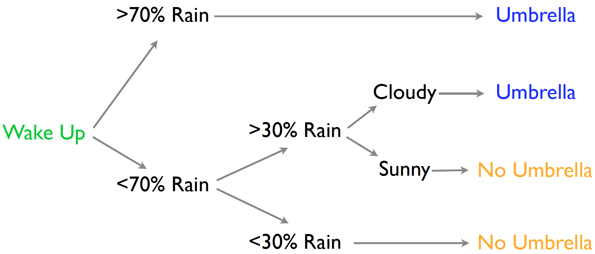
- Tree-logic uses a series of steps to come to a conclusion.
- The trick is to have mini-decisions combine for good choices.
- Each decision is a node, and the final prediction is a leaf node.
Decision trees are useful for both classification and regression.
Decision trees can take any type of data, numerical or categorical.
Decision trees make fewer assumptions about the relationship between
xandy.- E.g., linear model assumes the linear relationship between
xandy. - Decision trees naturally express certain kinds of interactions among the input variables: those of the form “IF x is true AND y is true, THEN….”
- E.g., linear model assumes the linear relationship between
- Classification trees have class probabilities at the leaves.
- Probability I’ll be in heavy rain is 0.9 (so take an umbrella).
- Regression trees have a mean response at the leaves.
- The expected amount of rain is 2 inches (so take an umbrella).
- CART: Classification and Regression Trees.
- We need a way to estimate the sequence of decisions.
- How many are they?
- What is the order?
- CART grows the tree through a sequence of splits:
- Given any set (node) of data, we can find the optimal split (the error minimizing split) and divide into two child sets.
- We then look at each child set, and again find the optimal split to divide it into two homogeneous subsets.
- The children become parents, and we look again for the optimal split on their new children (the grandchildren!).
- We stop splitting and growing when the size of the leaf nodes hits some minimum threshold (e.g., say no less than 10 observations per leaf).
Objective at each split: find the best variable to partition the data into one of two regions, \(R_1\) & \(R_2\), to minimize the error between the actual response, \(y_i\), and the node’s predicted constant, \(c_i\)
- For regression we minimize the sum of squared errors (SSE):
\[ S S E=\sum_{i \in R_{1}}\left(y_{i}-c_{1}\right)^{2}+\sum_{i \in R_{2}}\left(y_{i}-c_{2}\right)^{2} \]
For classification trees we minimize the node’s impurity the Gini index
where \(p_k\) is the proportion of observations in the node belonging to class \(k\) out of \(K\) total classes
want to minimize \(Gini\): small values indicate a node has primarily one class (is more pure)
Gini impurity measures the degree of a particular variable being wrongly classified when it is randomly chosen.
\[ Gini = 1 - \sum_k^K p_k^2 \]
NBC Show Data
- The dataset (
nbcanddemog) is from NBC’s TV pilots:- Gross Ratings Points (GRP): estimated total viewership, which measures broadcast marketability.
- Projected Engagement (PE): a more suitable measure of audience.
- After watching a show, viewer is quizzed on order and detail.
- This measures their engagement with the show (and ads!).
library(tidyverse)
nbc <- read_csv('https://bcdanl.github.io/data/nbc_show.csv')
nbc$Genre <- as.factor(nbc$Genre)skim(nbc)| Name | nbc |
| Number of rows | 40 |
| Number of columns | 6 |
| _______________________ | |
| Column type frequency: | |
| character | 2 |
| factor | 1 |
| numeric | 3 |
| ________________________ | |
| Group variables | None |
Variable type: character
| skim_variable | n_missing | complete_rate | min | max | empty | n_unique | whitespace |
|---|---|---|---|---|---|---|---|
| Show | 0 | 1 | 4 | 34 | 0 | 40 | 0 |
| Network | 0 | 1 | 2 | 5 | 0 | 14 | 0 |
Variable type: factor
| skim_variable | n_missing | complete_rate | ordered | n_unique | top_counts |
|---|---|---|---|---|---|
| Genre | 0 | 1 | FALSE | 3 | Dra: 19, Rea: 17, Sit: 4 |
Variable type: numeric
| skim_variable | n_missing | complete_rate | mean | sd | p0 | p25 | p50 | p75 | p100 | hist |
|---|---|---|---|---|---|---|---|---|---|---|
| PE | 0 | 1 | 72.68 | 12.03 | 30.0 | 64.58 | 77.06 | 80.16 | 89.29 | ▁▁▃▃▇ |
| GRP | 0 | 1 | 823.90 | 683.42 | 7.5 | 301.45 | 647.90 | 1200.45 | 2773.80 | ▇▅▂▂▁ |
| Duration | 0 | 1 | 50.25 | 14.23 | 30.0 | 30.00 | 60.00 | 60.00 | 60.00 | ▃▁▁▁▇ |
ggplot(nbc) +
  geom_point(aes(x = GRP, y = PE, color = Genre),
             alpha = .75)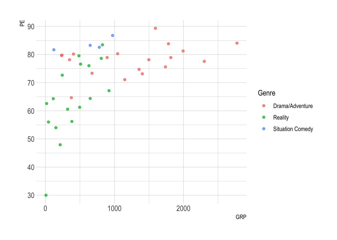
- Consider a classification tree to predict
Genrefrom demographics.- Output from tree shows a series of decision nodes and the proportion in each
Genreat these nodes, down to the leaves.
- Output from tree shows a series of decision nodes and the proportion in each
demog <- read_csv(
  'https://bcdanl.github.io/data/nbc_demog.csv'
)skim(demog)| Name | demog |
| Number of rows | 40 |
| Number of columns | 57 |
| _______________________ | |
| Column type frequency: | |
| character | 1 |
| numeric | 56 |
| ________________________ | |
| Group variables | None |
Variable type: character
| skim_variable | n_missing | complete_rate | min | max | empty | n_unique | whitespace |
|---|---|---|---|---|---|---|---|
| Show | 0 | 1 | 4 | 34 | 0 | 40 | 0 |
Variable type: numeric
| skim_variable | n_missing | complete_rate | mean | sd | p0 | p25 | p50 | p75 | p100 | hist |
|---|---|---|---|---|---|---|---|---|---|---|
| TERRITORY.EAST.CENTRAL | 0 | 1 | 13.51 | 2.78 | 6.16 | 11.73 | 14.05 | 15.36 | 19.98 | ▁▃▆▇▁ |
| TERRITORY.NORTHEAST | 0 | 1 | 20.35 | 3.17 | 14.01 | 18.04 | 20.31 | 22.49 | 27.80 | ▂▇▇▅▂ |
| TERRITORY.PACIFIC | 0 | 1 | 17.42 | 3.67 | 9.47 | 15.24 | 17.72 | 19.68 | 28.79 | ▃▃▇▁▁ |
| TERRITORY.SOUTHEAST | 0 | 1 | 21.56 | 3.68 | 16.23 | 19.21 | 21.32 | 22.92 | 37.11 | ▇▇▂▁▁ |
| TERRITORY.SOUTHWEST | 0 | 1 | 11.83 | 2.29 | 7.68 | 10.47 | 11.58 | 13.45 | 16.24 | ▃▇▇▅▅ |
| TERRITORY.WEST.CENTRAL | 0 | 1 | 15.33 | 3.15 | 9.64 | 12.99 | 15.01 | 16.93 | 22.69 | ▂▇▇▂▂ |
| COUNTY.SIZE.A | 0 | 1 | 39.27 | 6.01 | 28.36 | 35.14 | 39.55 | 42.75 | 51.55 | ▃▇▇▃▃ |
| COUNTY.SIZE.B | 0 | 1 | 32.14 | 3.29 | 22.30 | 30.65 | 32.04 | 33.69 | 38.60 | ▁▁▇▆▂ |
| COUNTY.SIZE.C | 0 | 1 | 14.67 | 2.73 | 8.24 | 13.00 | 14.66 | 16.37 | 20.55 | ▂▅▇▇▂ |
| COUNTY.SIZE.D | 0 | 1 | 13.93 | 3.80 | 4.47 | 11.92 | 14.11 | 16.60 | 24.95 | ▂▆▇▅▁ |
| WIRED.CABLE.W.PAY | 0 | 1 | 34.63 | 6.01 | 24.79 | 30.34 | 34.74 | 36.97 | 48.91 | ▅▅▇▂▂ |
| WIRED.CABLE.W.O.PAY | 0 | 1 | 29.58 | 5.33 | 21.95 | 25.73 | 28.45 | 34.24 | 43.60 | ▇▇▅▂▂ |
| DBS.OWNER | 0 | 1 | 23.60 | 4.85 | 10.03 | 20.47 | 24.85 | 26.50 | 31.83 | ▁▂▃▇▃ |
| BROADCAST.ONLY | 0 | 1 | 12.72 | 11.42 | 0.00 | 0.00 | 14.04 | 20.96 | 37.96 | ▇▃▆▂▁ |
| VIDEO.GAME.OWNER | 0 | 1 | 57.20 | 4.91 | 49.02 | 53.61 | 56.03 | 60.48 | 67.87 | ▂▇▃▂▂ |
| DVD.OWNER | 0 | 1 | 92.77 | 2.15 | 87.44 | 91.44 | 92.73 | 94.23 | 98.46 | ▁▇▇▇▁ |
| VCR.OWNER | 0 | 1 | 84.37 | 3.42 | 74.14 | 82.66 | 85.40 | 86.55 | 90.40 | ▁▁▃▇▂ |
| X1.TV.SET | 0 | 1 | 11.53 | 3.28 | 1.54 | 9.90 | 11.11 | 13.95 | 19.30 | ▁▂▇▂▂ |
| X2.TV.SETS | 0 | 1 | 27.03 | 2.71 | 21.72 | 25.29 | 27.18 | 28.49 | 34.05 | ▂▆▇▃▁ |
| X3.TV.SETS | 0 | 1 | 28.37 | 3.43 | 21.72 | 26.53 | 28.14 | 29.67 | 39.85 | ▂▇▅▁▁ |
| X4..TV.SETS | 0 | 1 | 33.08 | 3.41 | 27.48 | 31.14 | 32.64 | 34.70 | 43.72 | ▃▇▃▁▁ |
| X1.PERSON | 0 | 1 | 10.92 | 3.54 | 1.78 | 9.16 | 10.90 | 12.99 | 21.98 | ▁▃▇▂▁ |
| X2.PERSONS | 0 | 1 | 25.15 | 2.69 | 19.54 | 23.32 | 25.43 | 26.58 | 30.58 | ▃▃▇▇▃ |
| X3.PERSONS | 0 | 1 | 22.84 | 2.00 | 18.85 | 21.61 | 22.61 | 23.62 | 28.41 | ▂▇▆▂▂ |
| X4..PERSONS | 0 | 1 | 41.09 | 4.72 | 28.41 | 39.12 | 40.59 | 42.96 | 56.75 | ▁▇▇▂▁ |
| HOH..25 | 0 | 1 | 6.52 | 3.78 | 0.83 | 4.34 | 6.00 | 7.96 | 20.36 | ▆▇▂▁▁ |
| HOH.25.34 | 0 | 1 | 25.07 | 4.75 | 16.17 | 21.21 | 26.06 | 28.69 | 32.47 | ▅▃▅▇▅ |
| HOH.35.44 | 0 | 1 | 33.70 | 4.58 | 19.13 | 31.34 | 33.93 | 36.08 | 45.02 | ▁▁▇▆▁ |
| HOH.45.54 | 0 | 1 | 26.01 | 4.17 | 14.76 | 23.03 | 25.59 | 28.89 | 33.18 | ▁▂▇▅▅ |
| HOH.55.64 | 0 | 1 | 5.70 | 1.60 | 2.49 | 4.40 | 6.00 | 7.00 | 8.37 | ▃▆▅▇▆ |
| HOH.65. | 0 | 1 | 3.01 | 1.09 | 0.55 | 2.46 | 3.03 | 3.85 | 4.92 | ▁▅▇▅▃ |
| X1.3.YRS.COLLEGE | 0 | 1 | 32.90 | 2.70 | 26.18 | 31.67 | 32.63 | 34.39 | 41.94 | ▂▇▇▁▁ |
| X4..YRS.COLLEGE | 0 | 1 | 29.72 | 8.94 | 11.16 | 24.29 | 29.54 | 35.60 | 47.39 | ▂▃▇▃▂ |
| X4.YRS.H.S. | 0 | 1 | 29.50 | 5.90 | 16.22 | 25.11 | 29.68 | 33.23 | 42.57 | ▂▅▇▅▂ |
| WHITE.COLLAR | 0 | 1 | 50.85 | 7.38 | 30.92 | 47.97 | 51.62 | 56.47 | 60.99 | ▁▃▅▇▇ |
| BLUE.COLLAR | 0 | 1 | 30.20 | 4.93 | 22.05 | 27.63 | 29.59 | 32.95 | 46.99 | ▃▇▃▁▁ |
| NOT.IN.LABOR.FORCE | 0 | 1 | 18.95 | 4.66 | 8.86 | 16.08 | 17.57 | 22.09 | 31.64 | ▁▇▅▁▁ |
| BLACK | 0 | 1 | 14.00 | 5.66 | 2.56 | 10.74 | 12.90 | 16.48 | 35.34 | ▂▇▆▁▁ |
| WHITE | 0 | 1 | 78.54 | 7.03 | 53.96 | 75.71 | 78.21 | 83.15 | 91.53 | ▁▁▅▇▃ |
| OTHER | 0 | 1 | 7.46 | 2.29 | 4.06 | 5.98 | 6.65 | 8.55 | 12.58 | ▅▇▃▂▂ |
| ANY.CHILDREN.2.5 | 0 | 1 | 18.17 | 3.13 | 12.16 | 15.89 | 17.98 | 20.06 | 25.21 | ▃▅▇▃▂ |
| ANY.CHILDREN.6.11 | 0 | 1 | 22.75 | 3.98 | 13.64 | 21.03 | 22.70 | 24.60 | 36.49 | ▂▇▇▁▁ |
| ANY.CHILDREN.12.17 | 0 | 1 | 24.37 | 4.53 | 17.80 | 22.30 | 24.11 | 25.57 | 40.40 | ▃▇▁▁▁ |
| ANY.CATS | 0 | 1 | 33.98 | 3.76 | 26.32 | 31.31 | 33.98 | 36.49 | 41.59 | ▂▇▅▇▂ |
| ANY.DOGS | 0 | 1 | 48.46 | 4.47 | 36.77 | 46.77 | 48.53 | 50.67 | 62.94 | ▁▅▇▂▁ |
| MALE.HOH | 0 | 1 | 48.87 | 5.05 | 36.26 | 46.02 | 48.83 | 51.89 | 56.89 | ▂▂▇▇▆ |
| FEMALE.HOH | 0 | 1 | 51.14 | 5.06 | 43.10 | 48.12 | 51.13 | 53.99 | 63.97 | ▆▇▇▂▂ |
| INCOME.30.74K. | 0 | 1 | 41.74 | 3.55 | 31.04 | 40.23 | 41.48 | 43.64 | 54.32 | ▁▃▇▁▁ |
| INCOME.75K. | 0 | 1 | 37.22 | 8.82 | 20.11 | 29.95 | 37.78 | 43.89 | 56.87 | ▃▅▅▇▁ |
| HISPANIC.ORIGIN | 0 | 1 | 8.18 | 3.34 | 3.85 | 5.60 | 7.85 | 9.75 | 19.56 | ▇▆▂▁▁ |
| NON.HISPANIC.ORIGIN | 0 | 1 | 91.82 | 3.35 | 80.34 | 90.21 | 92.12 | 94.42 | 96.15 | ▁▁▂▆▇ |
| HOME.IS.OWNED | 0 | 1 | 70.27 | 7.56 | 52.59 | 67.42 | 73.01 | 75.54 | 80.88 | ▃▂▃▇▇ |
| HOME.IS.RENTED | 0 | 1 | 29.72 | 7.55 | 19.12 | 24.46 | 26.99 | 32.58 | 47.39 | ▇▇▃▂▃ |
| PC.NON.OWNER | 0 | 1 | 15.53 | 5.99 | 5.80 | 11.80 | 14.00 | 19.82 | 28.37 | ▃▇▃▃▂ |
| PC.OWNER.WITH.INTERNET.ACCESS | 0 | 1 | 75.70 | 7.65 | 59.35 | 70.90 | 77.11 | 80.58 | 88.17 | ▃▃▆▇▅ |
| PC.OWNER.WITHOUT.INTERNET.ACCESS | 0 | 1 | 8.77 | 2.57 | 2.03 | 7.29 | 8.35 | 9.78 | 15.20 | ▁▃▇▂▂ |
# install.packages(c("tree","randomForest","ranger", "rpart", "vip", "pdp", "caret"))
library(tree)
genretree <- tree(nbc$Genre ~ .,
                  data = demog[,-1],
                  mincut = 1)
nbc$genrepred <- predict(genretree,
                         newdata = demog[,-1],
                         type = "class")
# tree plot (dendrogram)
plot(genretree, col=8, lwd=2)
text(genretree, label="yprob")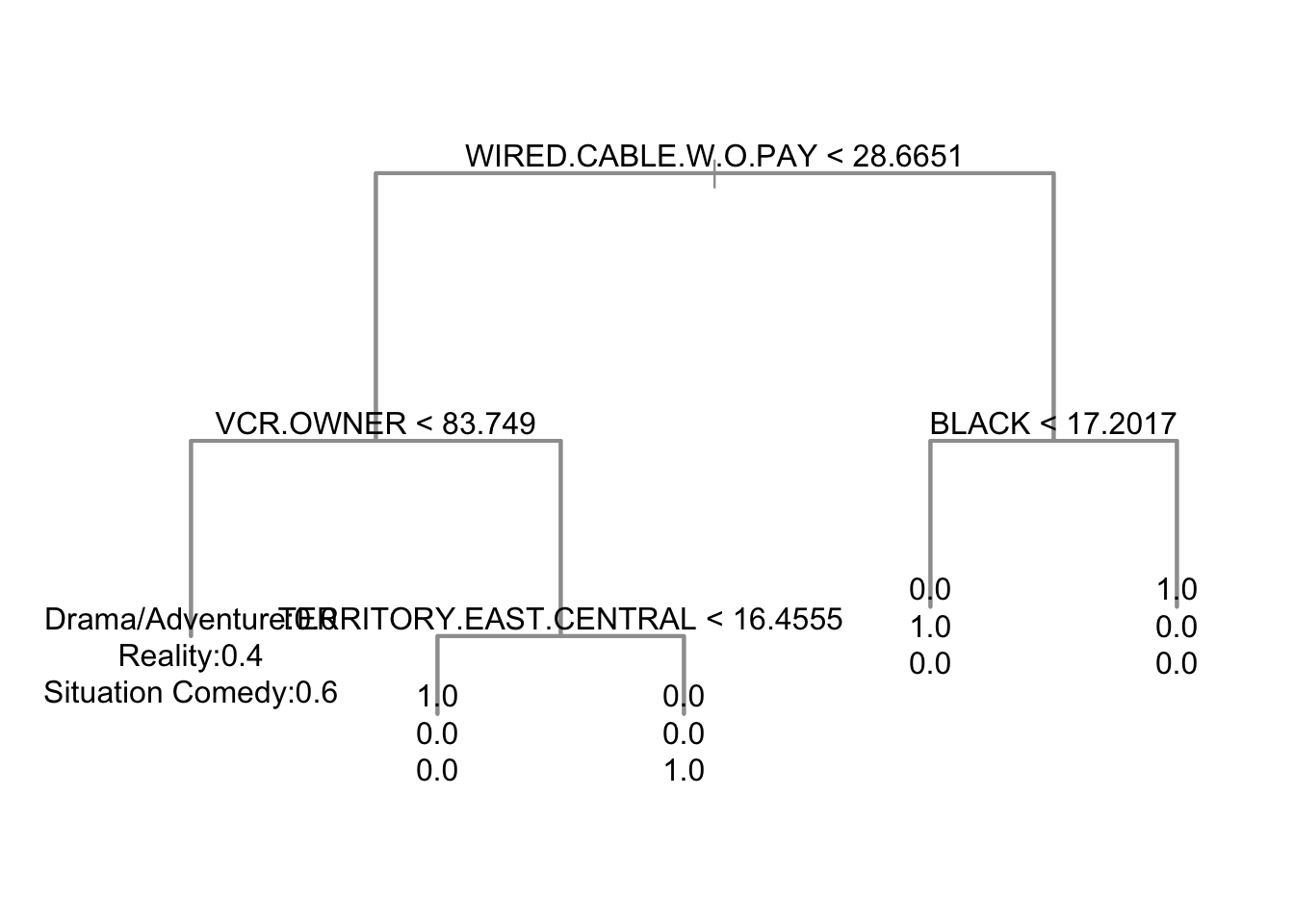
Consider predicting engagement from ratings and genre.
- Leaf predictions are expected engagement.
# mincut=1 allows for leaves containing a single show,
# with expected engagement that single show's PE.
nbctree <- tree(PE ~ Genre + GRP, data=nbc[,-1], mincut=1)
nbc$PEpred <- predict(nbctree, newdata=nbc[,-1])

## tree plot (dendrogram)
plot(nbctree, col=8, lwd=2)
text(nbctree)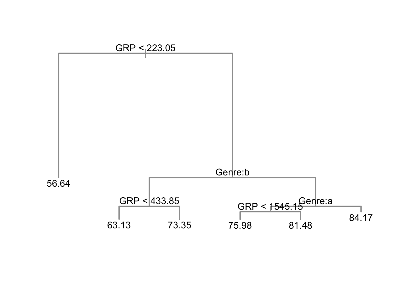
ggplot(nbc) +
  geom_point(aes(x = GRP, y = PE, color = Genre) ) +
  geom_line(aes(x = GRP, y = PEpred, color = Genre) )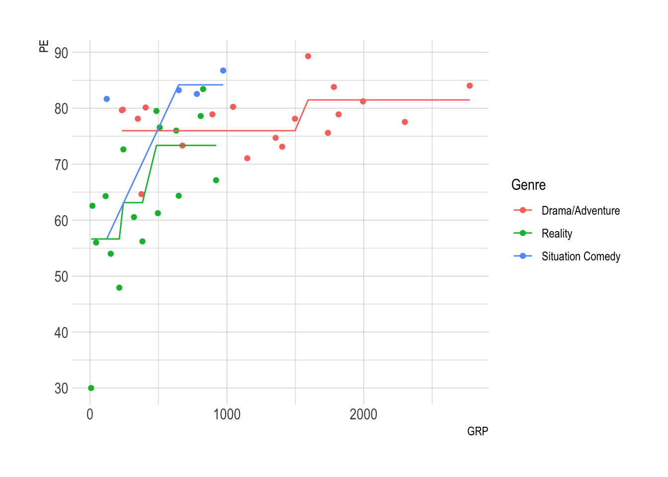
- PE increases with GRP, but in jumps!
CV Tree
- The biggest challenge with CART models is avoiding overfit.
- For CART, the usual solution is to rely on cross validation (CV).
- The way to cross-validate the fully fitted tree is to prune it by removing split rules from the bottom up:
- At each step, remove the split that contributes least to deviance reduction.
- This is a reverse to CART’s growth process.
- Pruning yields candidate tree.
- Each prune step produces a candidate tree model, and we can compare their out-of-sample prediction performance through CV.
Boston Housing Data
The
MASSpackage includes theBostondata.frame, which has 506 observations and 14 variables.crim: per capita crime rate by town.zn: proportion of residential land zoned for lots over 25,000 sq.ft.indus: proportion of non-retail business acres per town.chas: Charles River dummy variable (= 1 if tract bounds river; 0 otherwise).nox: nitrogen oxides concentration (parts per 10 million).rm: average number of rooms per dwelling.age: proportion of owner-occupied units built prior to 1940.dis: weighted mean of distances to five Boston employment centres.rad: index of accessibility to radial highways.tax: full-value property-tax rate per $10,000.ptratio: pupil-teacher ratio by town.black: \(1000(Bk - 0.63)^2\) where \(Bk\) is the proportion of blacks by town.lstat: lower status of the population (percent).medv: median value of owner-occupied homes in $1000s.
For more details about the data set, try
?Boston.The goal is to predict housing values.
library(MASS)
?Boston
Boston <- MASS::Bostonskim(MASS::Boston)| Name | MASS::Boston |
| Number of rows | 506 |
| Number of columns | 14 |
| _______________________ | |
| Column type frequency: | |
| numeric | 14 |
| ________________________ | |
| Group variables | None |
Variable type: numeric
| skim_variable | n_missing | complete_rate | mean | sd | p0 | p25 | p50 | p75 | p100 | hist |
|---|---|---|---|---|---|---|---|---|---|---|
| crim | 0 | 1 | 3.61 | 8.60 | 0.01 | 0.08 | 0.26 | 3.68 | 88.98 | ▇▁▁▁▁ |
| zn | 0 | 1 | 11.36 | 23.32 | 0.00 | 0.00 | 0.00 | 12.50 | 100.00 | ▇▁▁▁▁ |
| indus | 0 | 1 | 11.14 | 6.86 | 0.46 | 5.19 | 9.69 | 18.10 | 27.74 | ▇▆▁▇▁ |
| chas | 0 | 1 | 0.07 | 0.25 | 0.00 | 0.00 | 0.00 | 0.00 | 1.00 | ▇▁▁▁▁ |
| nox | 0 | 1 | 0.55 | 0.12 | 0.38 | 0.45 | 0.54 | 0.62 | 0.87 | ▇▇▆▅▁ |
| rm | 0 | 1 | 6.28 | 0.70 | 3.56 | 5.89 | 6.21 | 6.62 | 8.78 | ▁▂▇▂▁ |
| age | 0 | 1 | 68.57 | 28.15 | 2.90 | 45.02 | 77.50 | 94.07 | 100.00 | ▂▂▂▃▇ |
| dis | 0 | 1 | 3.80 | 2.11 | 1.13 | 2.10 | 3.21 | 5.19 | 12.13 | ▇▅▂▁▁ |
| rad | 0 | 1 | 9.55 | 8.71 | 1.00 | 4.00 | 5.00 | 24.00 | 24.00 | ▇▂▁▁▃ |
| tax | 0 | 1 | 408.24 | 168.54 | 187.00 | 279.00 | 330.00 | 666.00 | 711.00 | ▇▇▃▁▇ |
| ptratio | 0 | 1 | 18.46 | 2.16 | 12.60 | 17.40 | 19.05 | 20.20 | 22.00 | ▁▃▅▅▇ |
| black | 0 | 1 | 356.67 | 91.29 | 0.32 | 375.38 | 391.44 | 396.22 | 396.90 | ▁▁▁▁▇ |
| lstat | 0 | 1 | 12.65 | 7.14 | 1.73 | 6.95 | 11.36 | 16.96 | 37.97 | ▇▇▅▂▁ |
| medv | 0 | 1 | 22.53 | 9.20 | 5.00 | 17.02 | 21.20 | 25.00 | 50.00 | ▂▇▅▁▁ |
- Spliting training and testing data
set.seed(42120532)
index <- sample(nrow(Boston),nrow(Boston)*0.80)
Boston.train <- Boston[index,]
Boston.test <- Boston[-index,]- A bit of data visualization
Boston_vis <- Boston %>%
  gather(-medv, key = "var", value = "value") %>%
  filter(var != "chas")

ggplot(Boston_vis, aes(x = value, y = medv)) +
  geom_point(alpha = .33) +
  geom_smooth() +
facet_wrap(~ var, scales = "free") 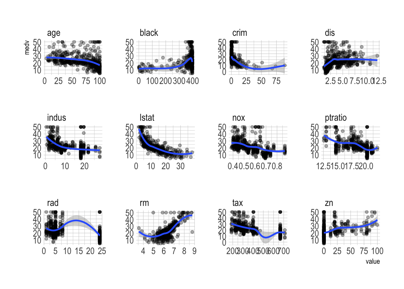
ggplot(Boston_vis, aes(y = value)) +
  geom_boxplot(outlier.color = "red", outlier.shape = 1) +
facet_wrap(~ var, scales = "free") 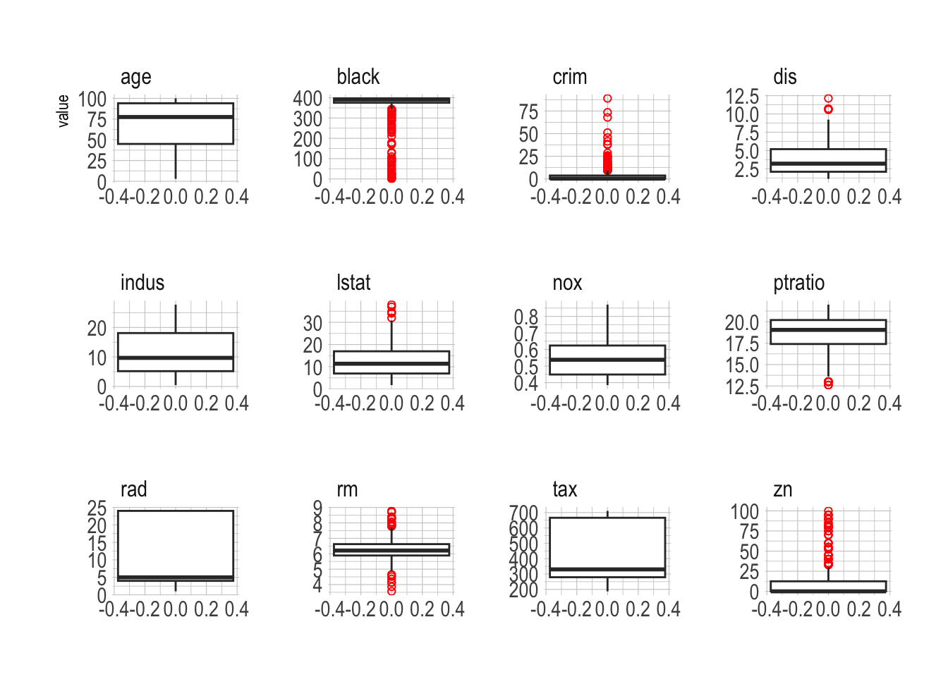
ggplot(Boston_vis, aes(x = value)) +
  geom_histogram() +
facet_wrap(~ var, scales = "free") 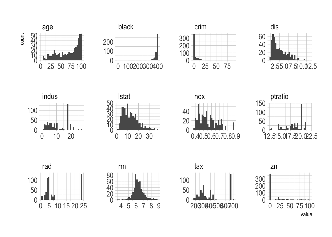
rpart()- Runs 10-fold CV tree to tune \(\alpha\) (CP) for pruning.
- Selects the number of terminal nodes via 1-SE rule.
library(rpart)
boston_tree <- rpart(medv ~ .,
                     data = Boston.train, method  = "anova")
boston_tree
n= 404
node), split, n, deviance, yval
* denotes terminal node
1) root 404 34343.3600 22.47178
2) lstat>=9.725 237 5424.9600 17.30084
4) lstat>=18.825 67 1000.6320 12.28358
8) nox>=0.603 51 417.5804 10.88039 *
9) nox< 0.603 16 162.5594 16.75625 *
5) lstat< 18.825 170 2073.0290 19.27824
10) lstat>=14.395 73 656.7096 17.12877 *
11) lstat< 14.395 97 825.2184 20.89588 *
3) lstat< 9.725 167 13588.0500 29.81018
6) rm< 7.4525 143 5781.9690 27.19790
12) dis>=1.95265 135 3329.1170 26.35185
24) rm< 6.722 88 927.6799 23.74886 *
25) rm>=6.722 47 688.8094 31.22553 *
13) dis< 1.95265 8 725.5350 41.47500 *
7) rm>=7.4525 24 1015.9250 45.37500 *printcpdisplayscptable for Fittedrpart()object:
printcp(boston_tree)
Regression tree:
rpart(formula = medv ~ ., data = Boston.train, method = "anova")

Variables actually used in tree construction:
[1] dis   lstat nox   rm

Root node error: 34343/404 = 85.008

n= 404

        CP nsplit rel error  xerror     xstd
1 0.446385      0   1.00000 1.00634 0.095395
2 0.197714      1   0.55362 0.65150 0.067953
3 0.068464      2   0.35590 0.39758 0.050182
4 0.050296      3   0.28744 0.32195 0.047053
5 0.049868      4   0.23714 0.32917 0.048158
6 0.017212      5   0.18727 0.29925 0.045811
7 0.012244      6   0.17006 0.27112 0.046339
8 0.010000 7 0.15782 0.27249 0.046513rpart.plot()plots the estimated tree structure from anrpart()object.- With
method = "anova"(a continuous outcome variable), each node shows:- the predicted value;
- the percentage of observations in the node.
- With
library(rpart.plot)
rpart.plot(boston_tree)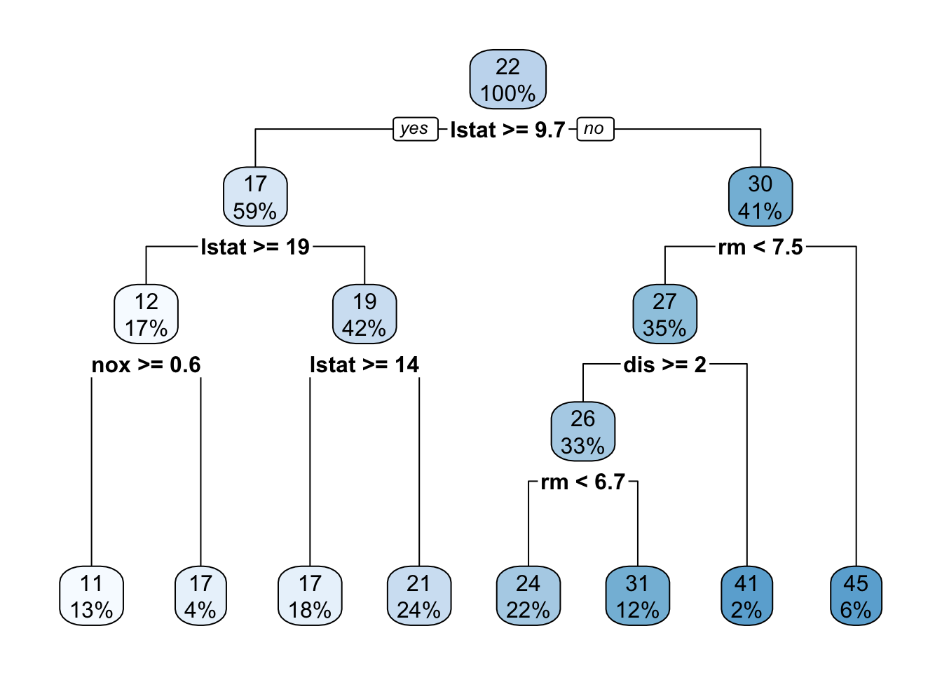
- With
method = "class"(a binary outcome variable), each node will show:- the predicted class;
- the predicted probability;
- the percentage of observations in the node.
plotcp()gives a visual representation of the cross-validation results in anrpart()object.- The size of a decision tree is the number of leaf nodes (non-terminal nodes) in the tree.
plotcp(boston_tree)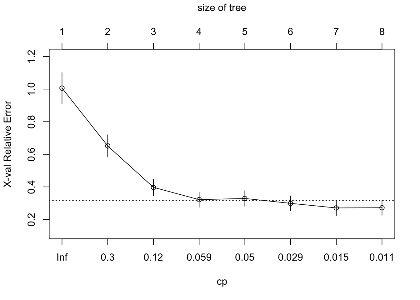
- What about the full tree? (
cp = 0)- The
controlparameter inrpart()allows for controlling therpartfit. (seerpart.fit)cp: complexity parameter. the minimum improvement in the model needed at each node.- The higher the
cp, the smaller the size of tree.
- The higher the
xval: number of cross-validations
- The
full_boston_tree <- rpart(formula = medv ~ .,
                       data = Boston.train, method  = "anova",
control = list(cp = 0, xval = 10))rpart.plot(full_boston_tree)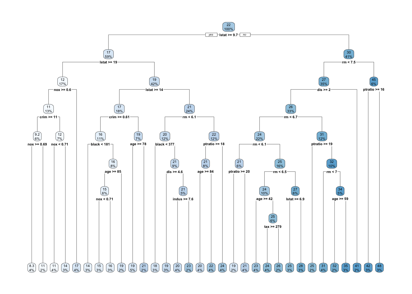
- Compare the full tree with the pruned tree.
- Which variable is not included in the pruned tree?
plotcp(full_boston_tree)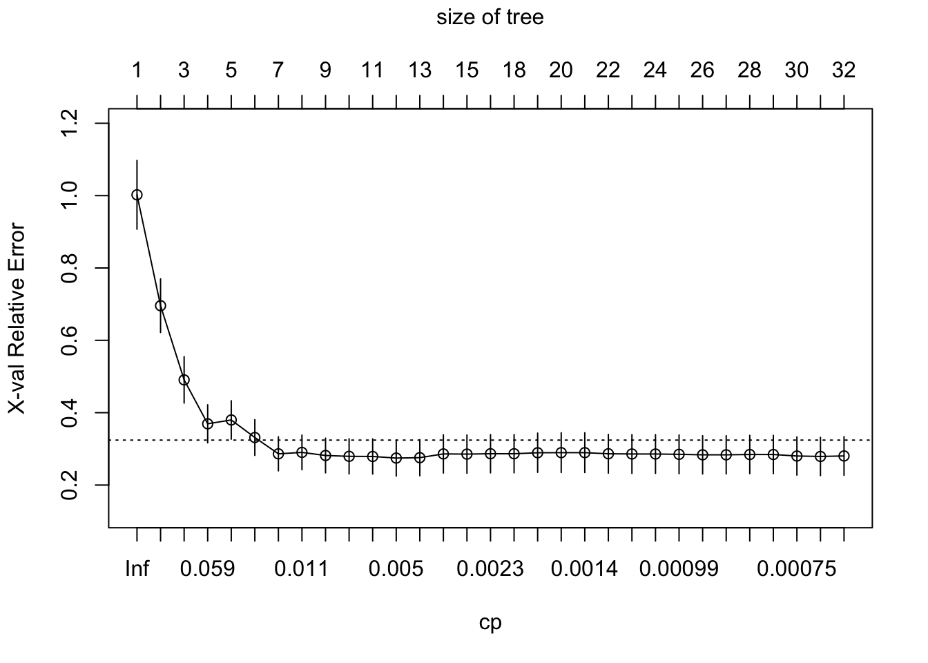
- We can train the CV trees with the
caretpackage as well:
library(caret)
caret_boston_tree <- train(medv ~ .,
                        data = Boston.train, method = "rpart",
                        trControl = trainControl(method = "cv", number = 10),
                        tuneLength = 20)
ggplot(caret_boston_tree)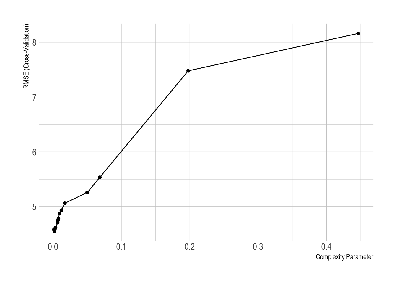
rpart.plot(caret_boston_tree$finalModel)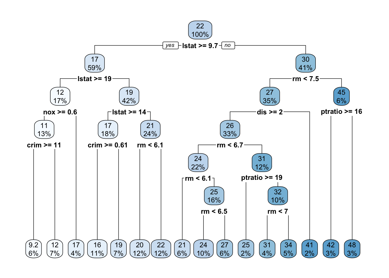
Random Forest
Why should we try other tree models?
- CART automatically learns non-linear response functions and will discover interactions between variables.
- Unfortunately, it is tough to avoid overfit with CART.
- High variance, i.e. split a dataset in half and grow tress in each half, the result will be very different
- CART generally results in higher test set error rates.
- Real structure of the tree is not easily chosen via cross-validation (CV).
- One way to mitigate the shortcomings of CART is bootstrap aggregation, or bagging.
Bagging Algorithm
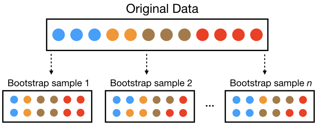
Bootstrap is random sampling with replacement.
Aggregation is combining the results from many trees together, each constructed with a different bootstrapped sample of the data.
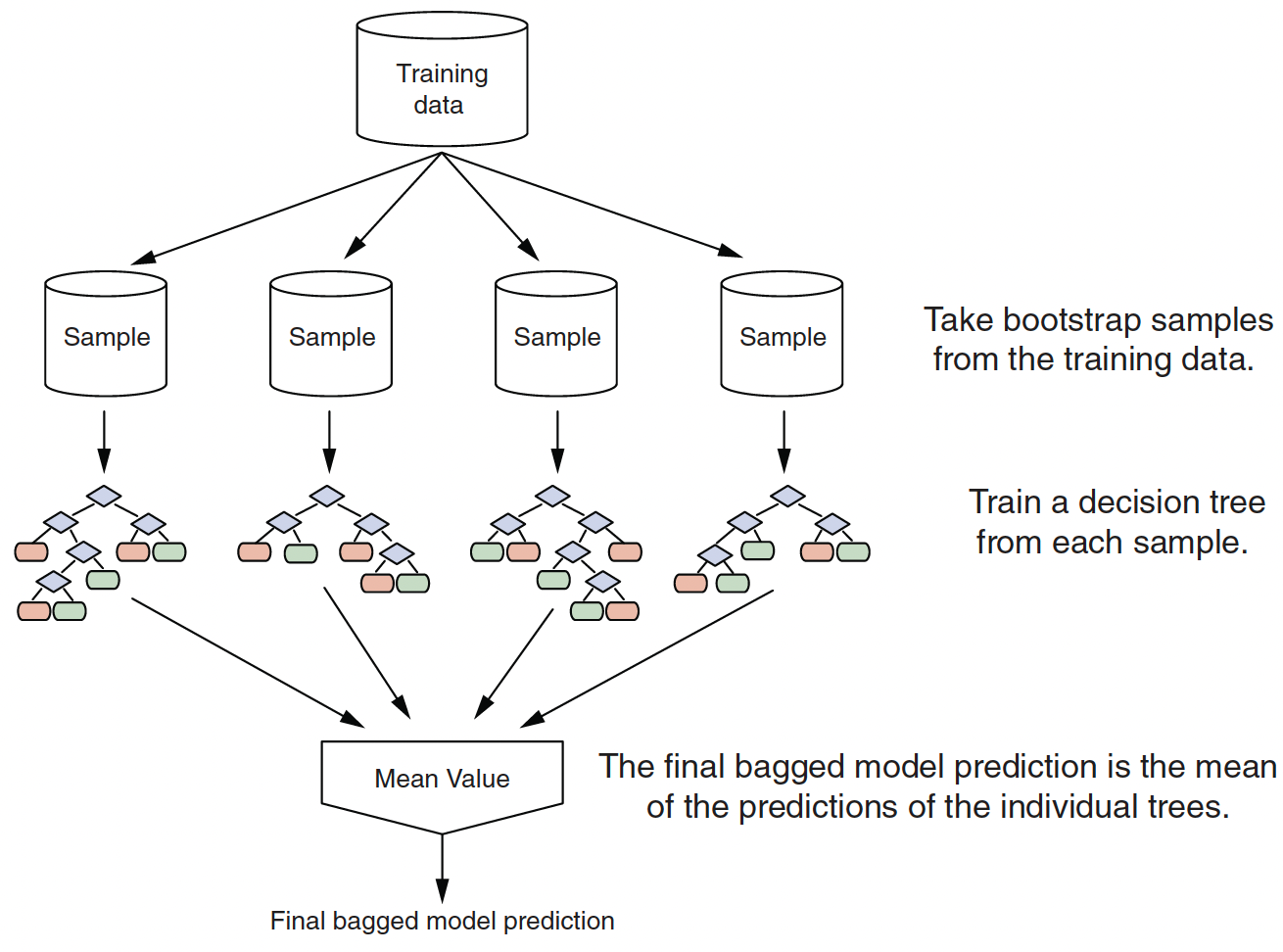
Real structure that persists across datasets shows up in the average.
A bagged ensemble of trees is also less likely to overfit the data.
To generate a prediction for a new point:
- Regression: take the average across the trees
- Classification: take the majority vote across the trees
- assuming each tree predicts a single class (could use probabilities instead…)
Bagging improves prediction accuracy via wisdom of the crowds but at the expense of interpretability.
- Easy to read one tree, but how do we read 500 trees?
- However, we can still use the measures of variable importance and partial dependence to summarize our models.
Random Forest Algorithm
- Random forests are an extension of bagging.
- At each split, the algorithm limits the variables considered to a random subset \(m_{try}\) of the given \(p\) number of variables.
- It introduce \(m_{try}\) as a tuning parameter: typically use \(p/3\) for regression or \(\sqrt{p}\) for classification.
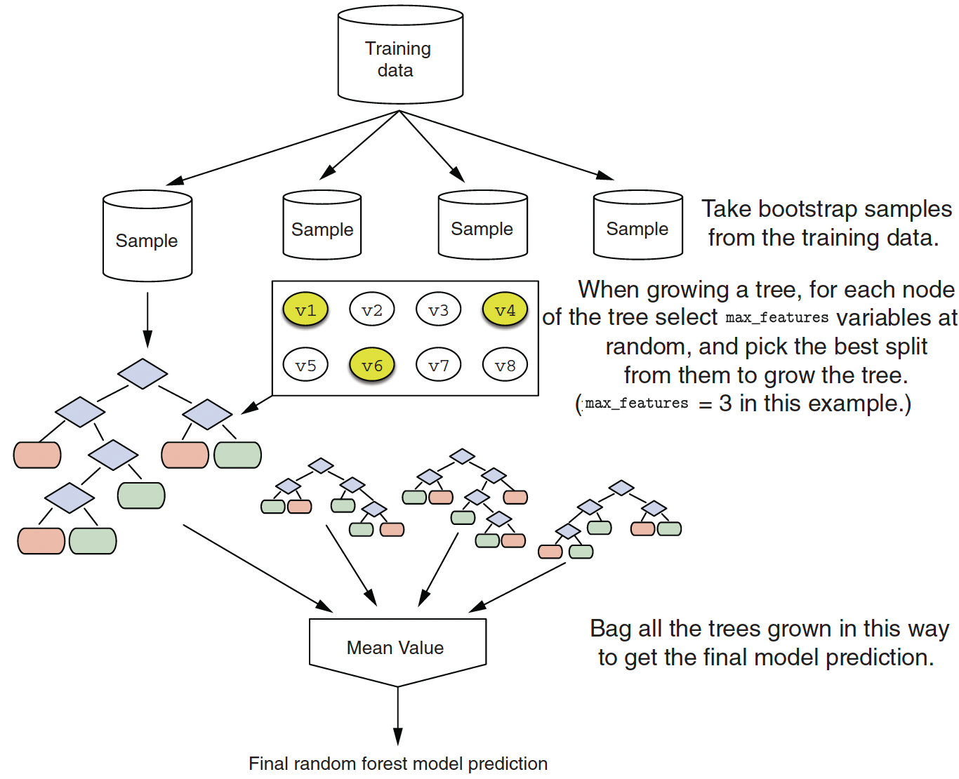
Split-variable randomization adds more randomness to make each tree more independent of each other.
The final ensemble of trees is bagged to make the random forest predictions.
Since the trees are constructed via bootstrapped data (samples with replacements), each sample is likely to have duplicate observations.
Out-of-bag (OOB), original observations not contained in a single bootstrap sample, can be used to make out-of-sample predictive performance of the model.
Intuition behind the Random Forest Algorithm
- The reason Random Forest algorithm considers a random subset of features at each split in the decision tree is to increase the diversity among the individual trees in the forest.
- This is a method to make the model more robust and prevent overfitting.
- If all the variables were considered at each split, each decision tree in the forest would look more similar, as they would likely use the same (or very similar) variables for splitting, especially the first few splits which typically have the most impact on the structure of the tree.
- This is because some features might be so informative that they would always be chosen for splits early in the tree construction process if all features were considered.
- This would make the trees in the forest correlated, which would reduce the power of the ensemble.
- By considering only a random subset of the variables at each split, we increase the chance that less dominant variables are considered, leading to a more diverse set of trees.
- This diversity is key to the power of the Random Forest algorithm, as it allows for a more robust prediction that is less likely to overfit the training data.
- It also helps to reduce the variance of the predictions, as the errors of the individual trees are likely to cancel each other out when averaged (for regression) or voted on (for classification).
rangerpackage is a popular & fast implementation (seerandomForestfor the original).- Let’s consider the estimation with
randomForestfirst.
- Let’s consider the estimation with
library(randomForest)
bag.boston <- randomForest(medv ~ ., data = Boston.train,
                           mtry=13, ntree = 50,
                           importance =TRUE)
bag.boston
Call:
 randomForest(formula = medv ~ ., data = Boston.train, mtry = 13,      ntree = 50, importance = TRUE)
               Type of random forest: regression
                     Number of trees: 50
No. of variables tried at each split: 13

          Mean of squared residuals: 10.94723
% Var explained: 87.12plot(bag.boston)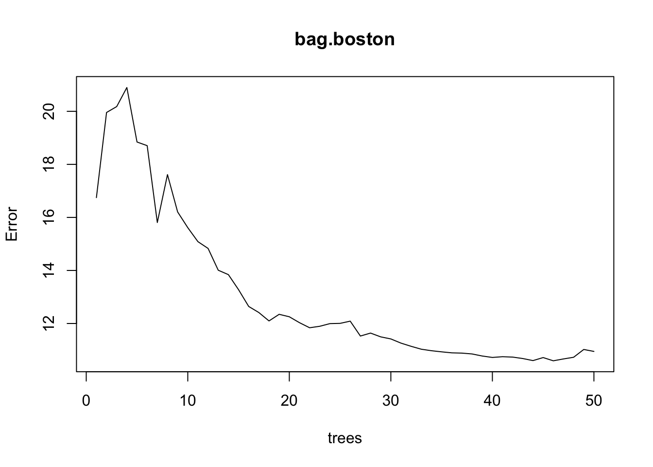
- Now Let’s consider the estimation with
ranger.
library(ranger)
bag.boston_ranger <- ranger(medv ~ ., data = Boston.train,
                            mtry = 13, num.trees = 50,
                            importance = "impurity")
bag.boston_ranger
Ranger result
Call:
ranger(medv ~ ., data = Boston.train, mtry = 13, num.trees = 50, importance = "impurity")
Type: Regression
Number of trees: 50
Sample size: 404
Number of independent variables: 13
Mtry: 13
Target node size: 5
Variable importance mode: impurity
Splitrule: variance
OOB prediction error (MSE): 10.58043
R squared (OOB): 0.8758446 CV Tree vs. Random Forest
We can compare the performance of the CV CART and the RF via MSE.
MSE from CV Tree
# prediction
boston.train.pred.CART <- predict(boston_tree, Boston.train)
boston.test.pred.CART <- predict(boston_tree, Boston.test)

# MSE
mean((Boston.test$medv - boston.test.pred.CART)^2)
[1] 22.94158mean((Boston.train$medv - boston.train.pred.CART)^2)[1] 13.41588- MSE from Random Forest
# prediction
boston.train.pred.RF <- predict(bag.boston_ranger, Boston.train)$predictions
boston.test.pred.RF <- predict(bag.boston_ranger, Boston.test)$predictions

# MSE
mean((Boston.test$medv - boston.test.pred.RF)^2)
[1] 11.24414mean((Boston.train$medv - boston.train.pred.RF)^2)[1] 1.987043Variable Importance in the Tree-based Models
- Variable importance is measured based on reduction in SSE.
- Mean Decrease Accuracy (% increase in MSE): This shows how much our model accuracy decreases if we leave out that variable.
- Mean Decrease Gini (Increase in Node Purity) : This is a measure of variable importance based on the Gini impurity index used for the calculating the splits in trees.
- Out-of-bag samples for datum
x1
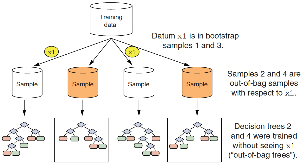
- Calculating variable importance of variable
v1
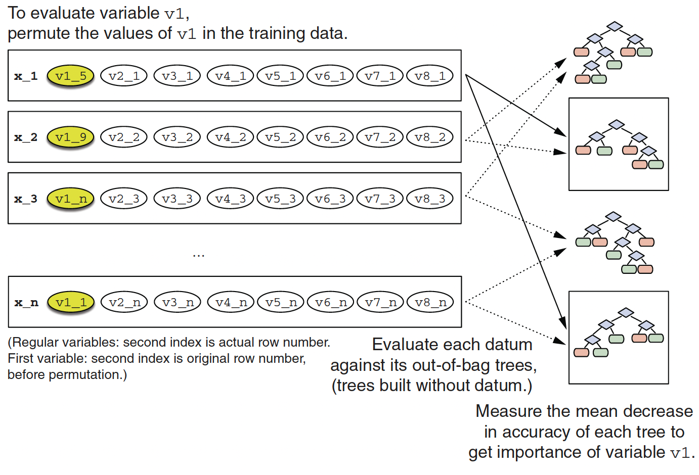
- Since we set
importancenot to equal to"none"when usingrpart,caret, andranger, we can evaluate variable importance using the left-out sample.
vip(caret_boston_tree, geom = "point")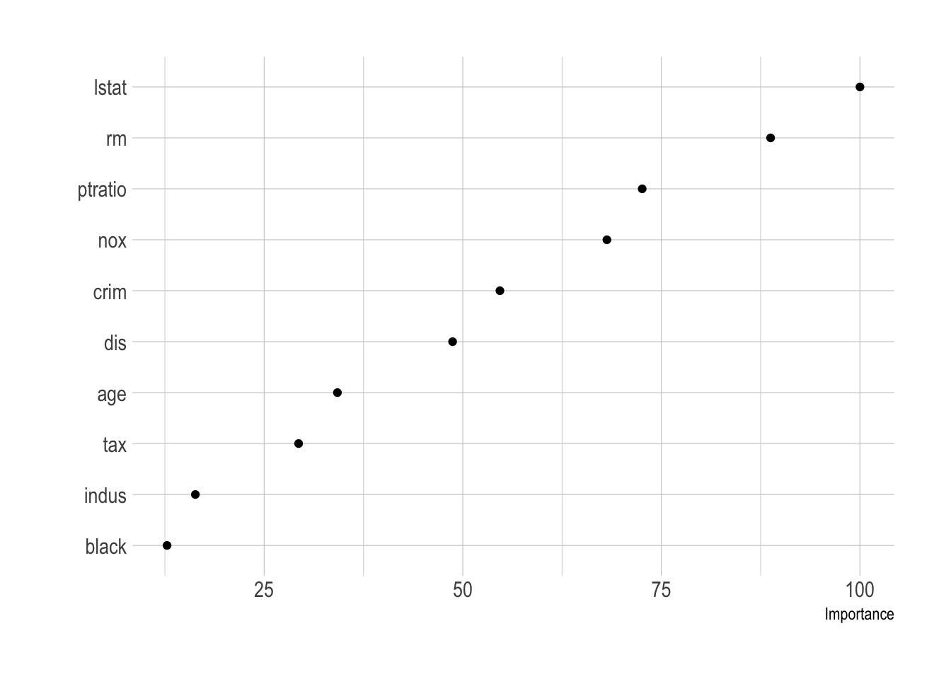
vip(full_boston_tree, geom = "point")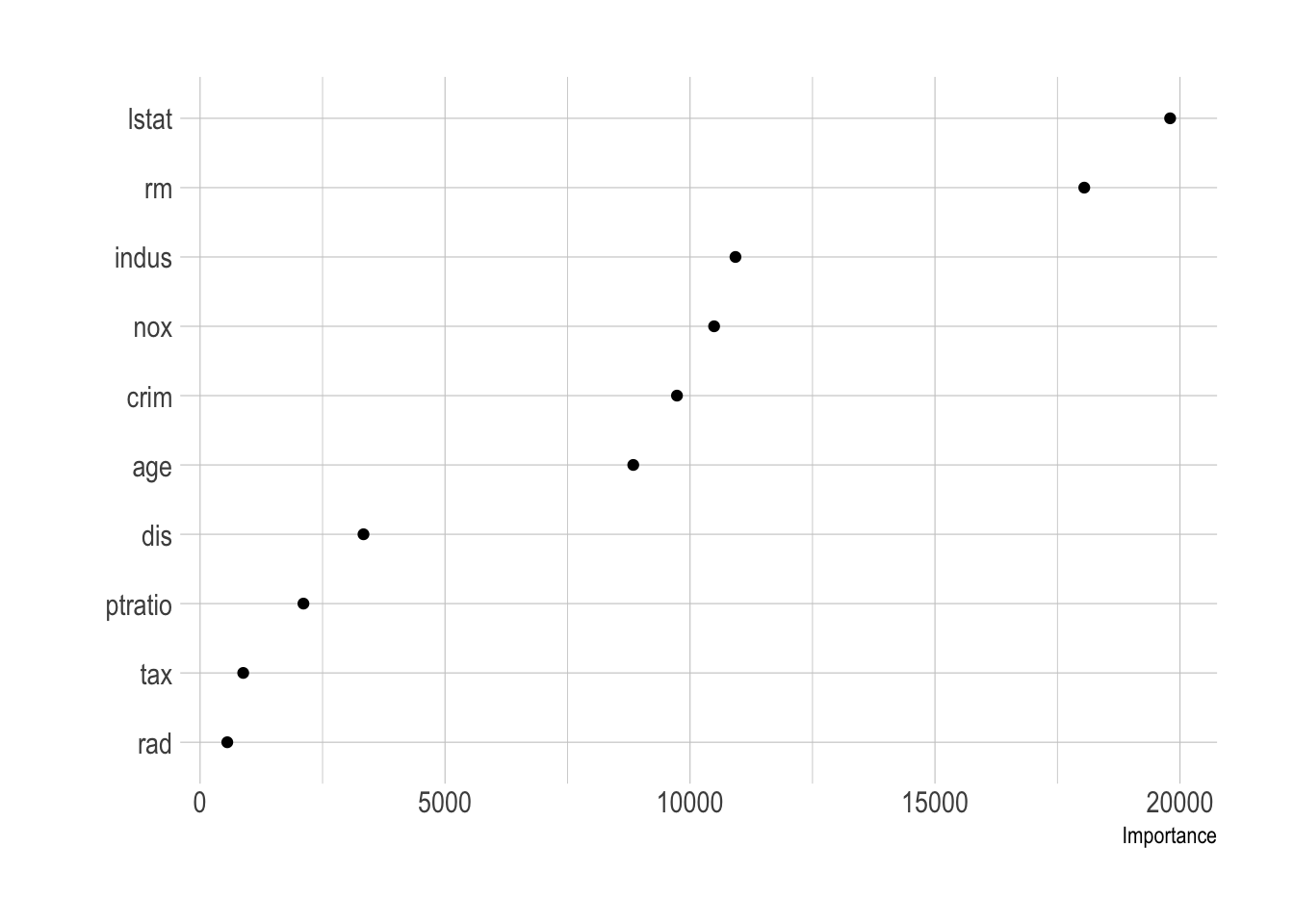
vip(boston_tree, geom = "point")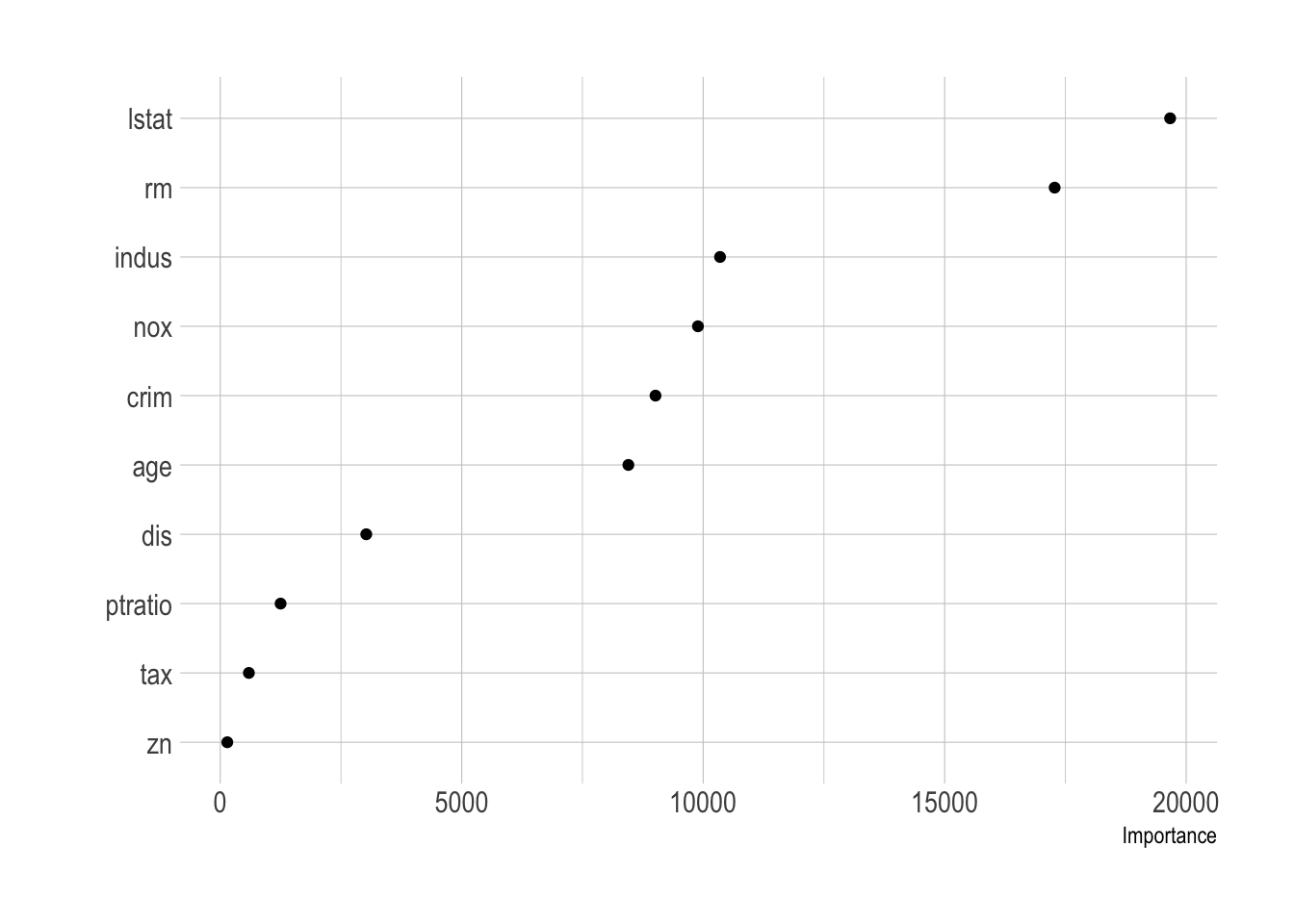
vip(bag.boston_ranger, geom = "point")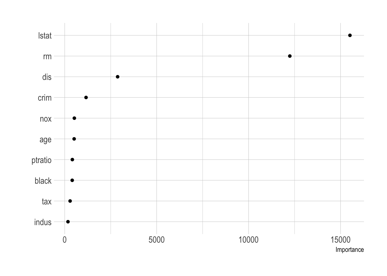
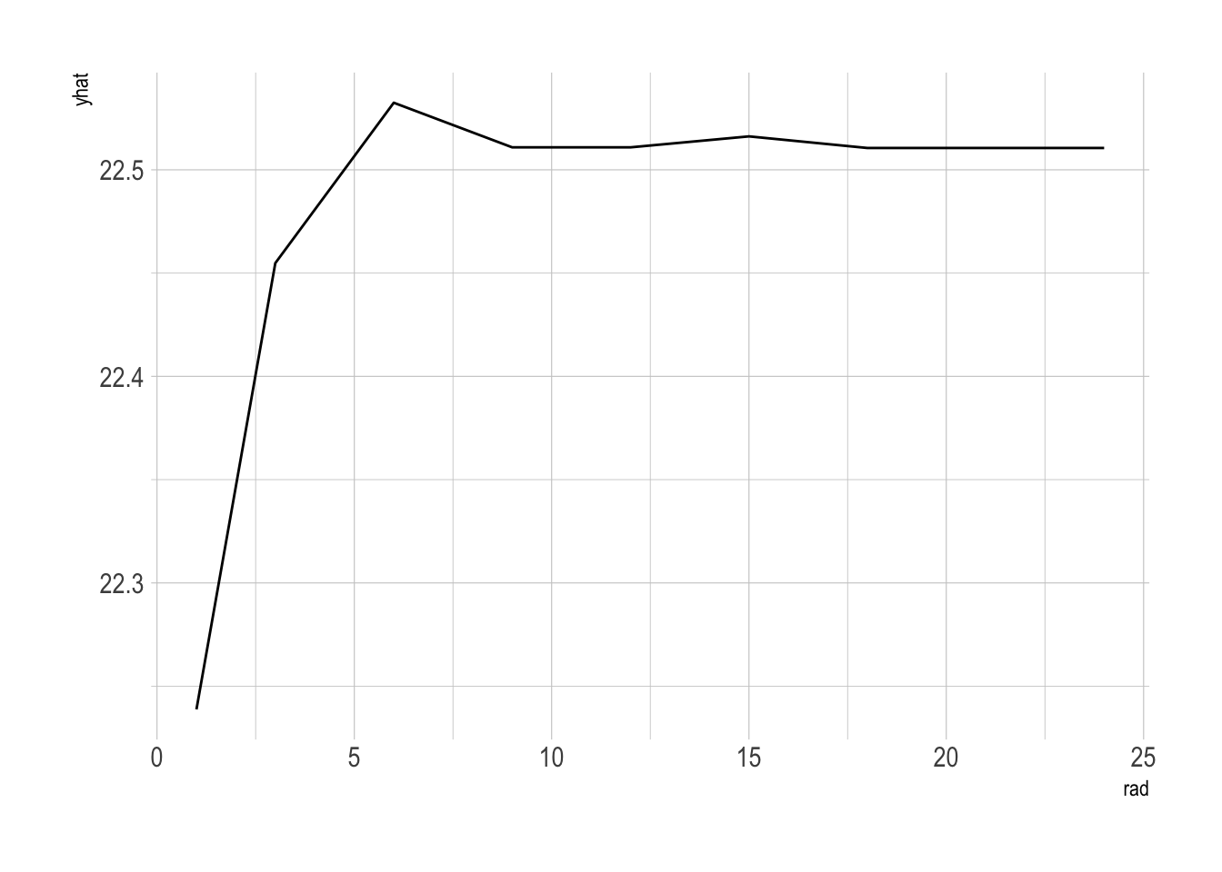
- We can also summarize the relationship between a predictor and the predicted outcome using a partial dependence plot
library(pdp)
# predictor, lstat
partial(bag.boston_ranger, pred.var = "lstat") %>% autoplot()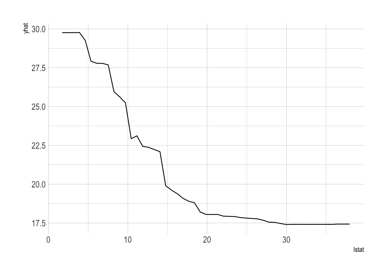
# predictor, rm
partial(bag.boston_ranger, pred.var = "rm") %>% autoplot()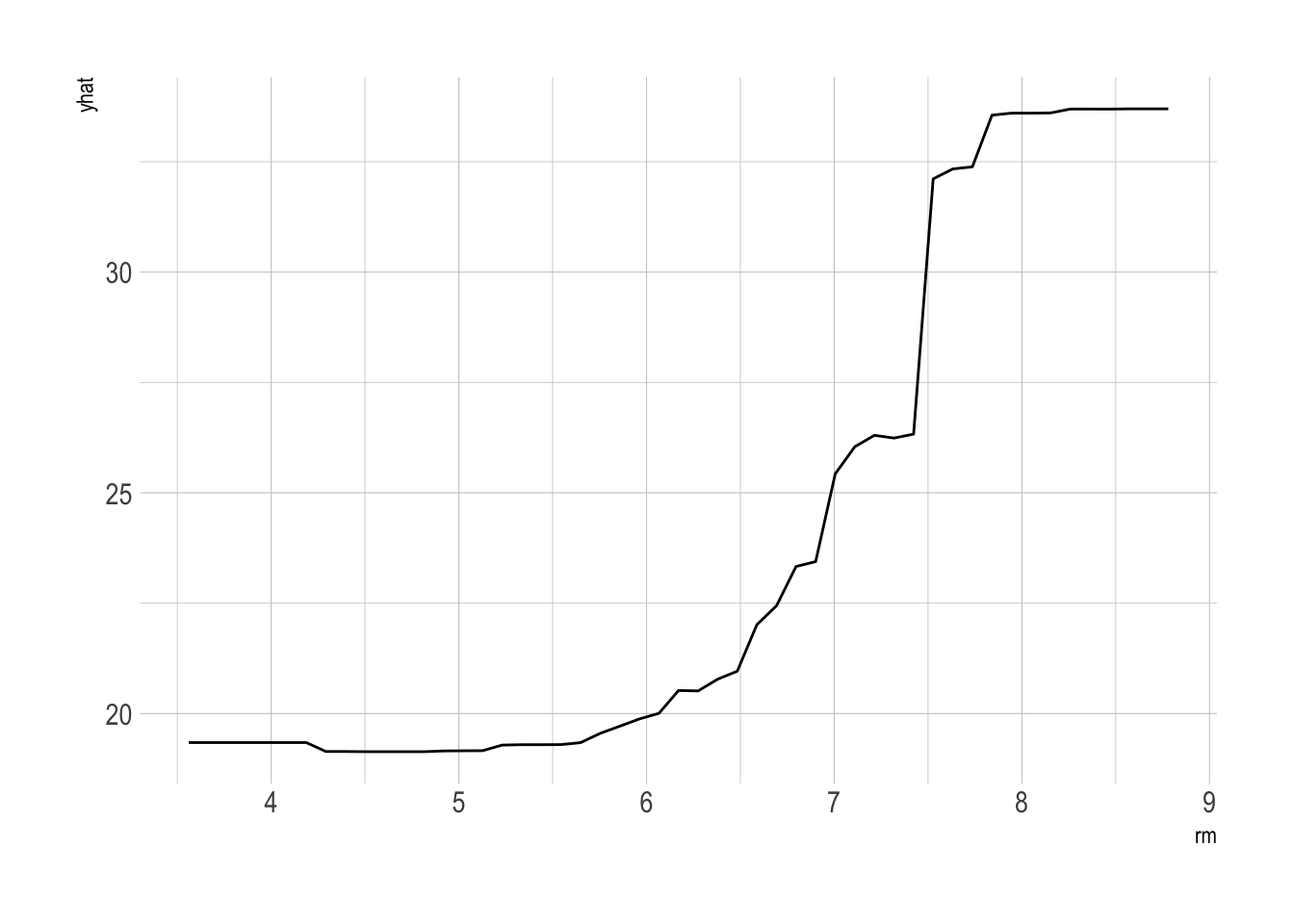
# predictor, rad
partial(bag.boston_ranger, pred.var = "rad") %>% autoplot()