Linear Regression

Machine Learning Lab

Author

Byeong-Hak Choe

Modified

May 8, 2024

Loading Packages and Data

library(tidyverse)
library(skimr) 
library(ggfortify) # to create regression-related plots
library(ggcorrplot) # to create correlation heatmaps
library(fastDummies) # to create dummy variables
library(stargazer) # to create regression tables

oj <- read_csv('https://bcdanl.github.io/data/dominick_oj.csv')

Exploratory Data Analysis

Descriptive Statistics

skim(oj)

Data summary
Name	oj
Number of rows	28947
Number of columns	4
_______________________
Column type frequency:
character	1
numeric	3
________________________
Group variables	None

Variable type: character

skim_variable	n_missing	complete_rate	min	max	empty	n_unique	whitespace
brand	0	1	9	11	0	3	0

Variable type: numeric

skim_variable	complete_rate	mean	sd	p0	p25	p50	p75	p100	hist
sales	1	17312.21	27477.66	64.00	4864.00	8384.00	17408.00	716416.00	▇▁▁▁▁
price	1	2.28	0.65	0.52	1.79	2.17	2.73	3.87	▁▆▇▅▂
ad	1	0.24	0.43	0.00	0.00	0.00	0.00	1.00	▇▁▁▁▂

oj %>% group_by(brand) %>% 
  skim()

Data summary
Name	Piped data
Number of rows	28947
Number of columns	4
_______________________
Column type frequency:
numeric	3
________________________
Group variables	brand

Variable type: numeric

skim_variable	brand	complete_rate	mean	sd	p0	p25	p50	p75	p100	hist
sales	dominicks	1	19834.56	32245.47	64.00	4416.00	9152.00	21056.00	716416.00	▇▁▁▁▁
sales	minute.maid	1	18238.46	29992.21	320.00	4800.00	8320.00	18560.00	591360.00	▇▁▁▁▁
sales	tropicana	1	13863.62	17515.82	192.00	5248.00	8000.00	13824.00	288384.00	▇▁▁▁▁
price	dominicks	1	1.74	0.39	0.52	1.58	1.59	1.99	2.69	▁▂▇▃▂
price	minute.maid	1	2.24	0.40	0.88	1.99	2.17	2.49	3.17	▁▂▇▆▂
price	tropicana	1	2.87	0.55	1.29	2.49	2.99	3.19	3.87	▁▃▅▇▅
ad	dominicks	1	0.26	0.44	0.00	0.00	0.00	1.00	1.00	▇▁▁▁▃
ad	minute.maid	1	0.29	0.45	0.00	0.00	0.00	1.00	1.00	▇▁▁▁▃
ad	tropicana	1	0.17	0.37	0.00	0.00	0.00	0.00	1.00	▇▁▁▁▂

oj %>% group_by(brand, ad) %>% 
  skim()

Data summary
Name	Piped data
Number of rows	28947
Number of columns	4
_______________________
Column type frequency:
numeric	2
________________________
Group variables	brand, ad

Variable type: numeric

skim_variable	brand	ad	complete_rate	mean	sd	p0	p25	p50	p75	p100	hist
sales	dominicks	0	1	11733.91	15718.77	64.00	3584.00	7040.00	13312.00	248000.00	▇▁▁▁▁
sales	dominicks	1	1	43251.33	50930.45	64.00	11888.00	27744.00	54160.00	716416.00	▇▁▁▁▁
sales	minute.maid	0	1	8372.65	7701.69	320.00	4160.00	6272.00	9984.00	231808.00	▇▁▁▁▁
sales	minute.maid	1	1	42566.32	46260.27	1728.00	16576.00	29440.00	49808.00	591360.00	▇▁▁▁▁
sales	tropicana	0	1	10038.86	10246.02	192.00	4864.00	7168.00	11008.00	175872.00	▇▁▁▁▁
sales	tropicana	1	1	33047.02	29632.94	1408.00	10816.00	23808.00	46896.00	288384.00	▇▂▁▁▁
price	dominicks	0	1	1.80	0.38	0.52	1.58	1.69	1.99	2.69	▁▂▇▅▂
price	dominicks	1	1	1.56	0.34	0.89	1.39	1.58	1.59	2.69	▂▇▂▁▁
price	minute.maid	0	1	2.33	0.41	0.88	1.99	2.26	2.62	3.17	▁▂▇▇▃
price	minute.maid	1	1	2.02	0.30	0.99	1.99	1.99	2.19	2.81	▁▂▇▂▂
price	tropicana	0	1	2.97	0.51	1.32	2.59	2.99	3.39	3.87	▁▂▃▇▅
price	tropicana	1	1	2.39	0.46	1.29	1.99	2.39	2.79	3.59	▁▇▆▅▂

Data Visualization

Correlation heatmap is a great tool to start identifying which input variables are strongly correlated with an outcome variable.

# to convert a factor variable into indicators
oj_dummies <- dummy_cols(oj, select_columns = 'brand' ) %>% 
  select(-brand)

# the matrix of the correlation test p-values
p.mat <- cor_pmat(oj_dummies) 

# correlation heatmap with correlation values
ggcorrplot( cor(oj_dummies), lab = T,
            type = 'lower',
            colors = c("#2E74C0", "white", "#CB454A"),
            p.mat = p.mat) # p.values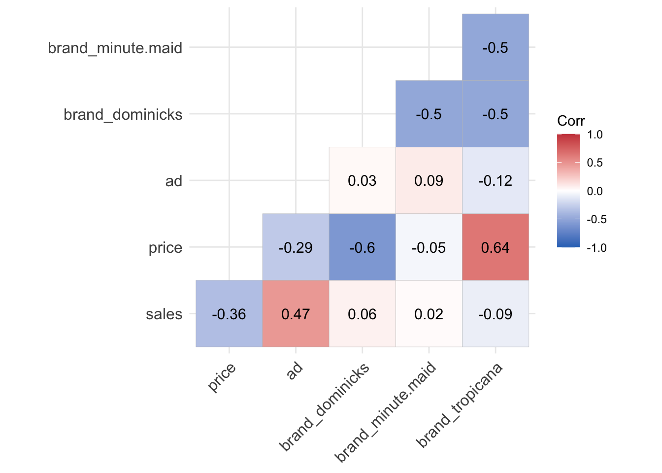

# variation in log price
ggplot(oj, aes(x = log(price), fill = brand )) +
  geom_histogram() +
  facet_wrap(brand ~., ncol = 1)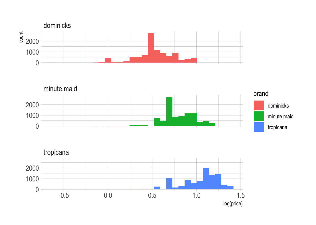

# variation in log sales
ggplot(oj, aes(x = log(sales), fill = brand )) +
  geom_histogram() +
  facet_wrap(brand ~., ncol = 1)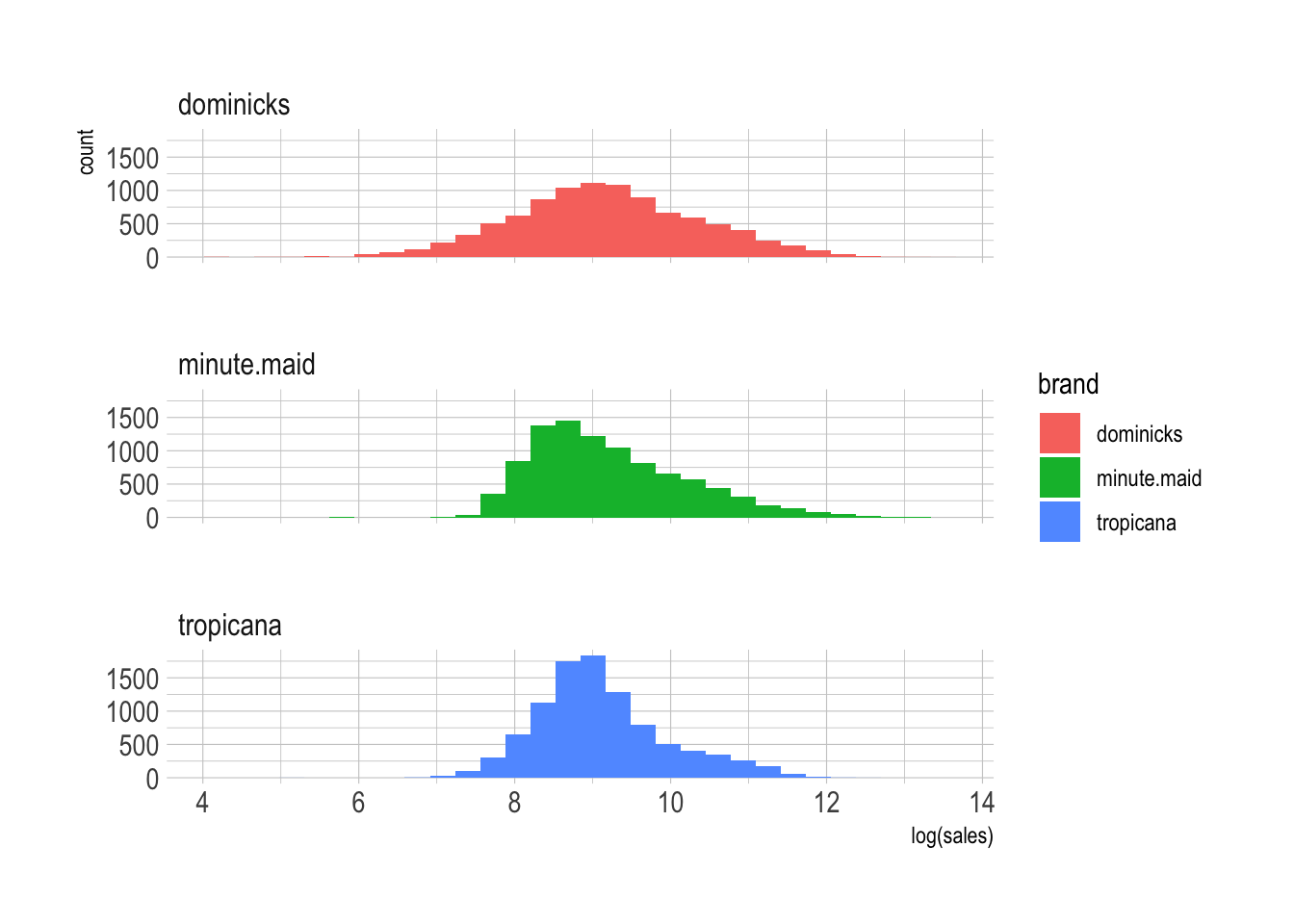

# law of demand
p <- ggplot(oj, aes(x = log(sales), y = log(price),
                    color = brand ))

p + geom_point( alpha = .025 ) +
  geom_smooth(method = lm, se = F)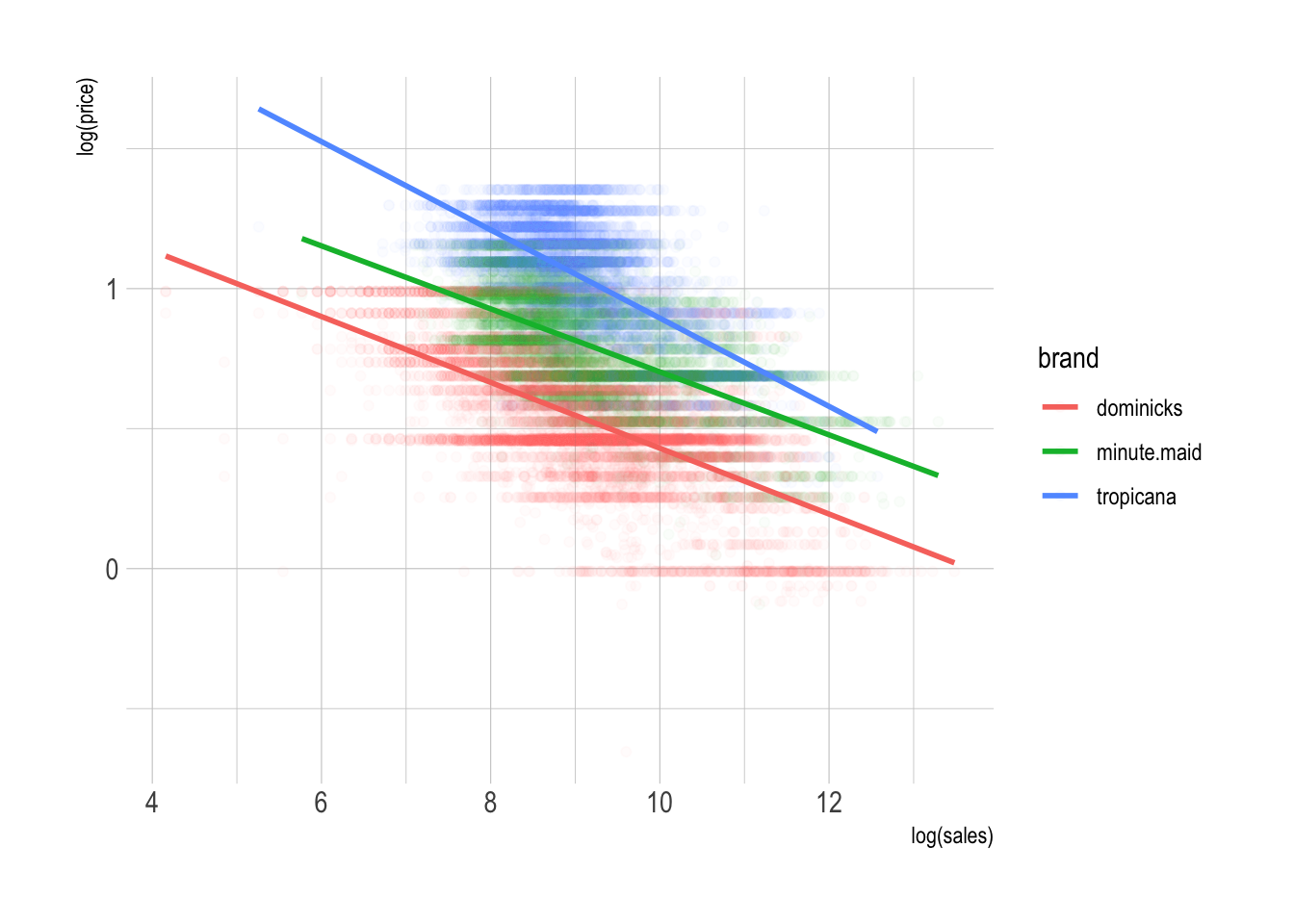

# mosaic plot
ggplot(data = oj) +
  geom_bar(aes(x = as.factor(ad), y = after_stat(prop),
               group = brand, fill = brand), 
           position = "fill") +
  labs(x = 'ad') +
  theme(plot.title = element_text(size = rel(1.5)),
        axis.title = element_text(size = 25),
        axis.text.x = element_text(size = rel(1.5)),
        axis.text.y = element_text(size = rel(1.5)))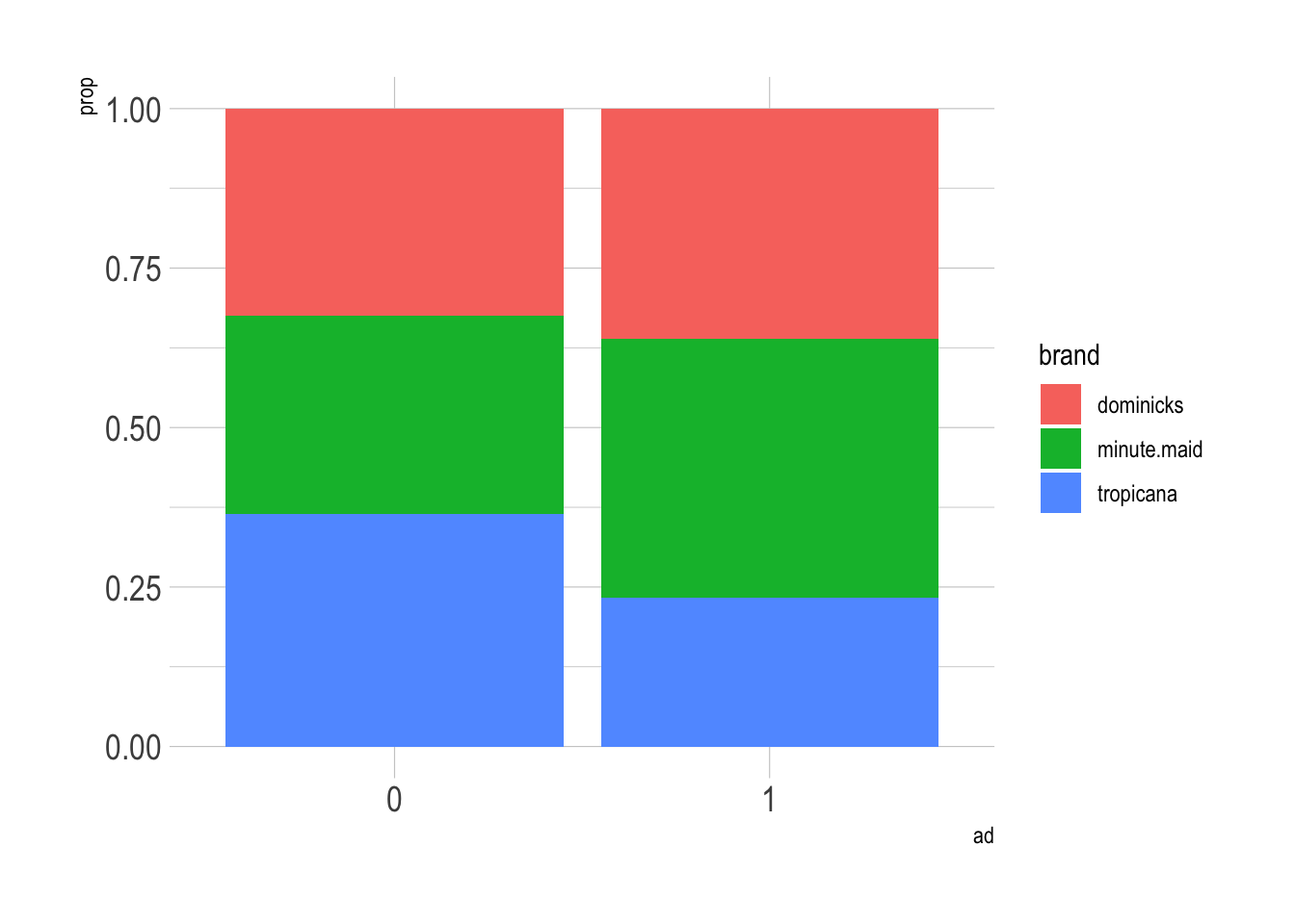

Linear Regression Model

A basic but powerful regression strategy is to deal in averages and lines.
- We model the conditional mean for $y$ given $x$ as

\[ \begin{align} \mathbb{E}[\, y \,|\, \mathbf{X} \,] &= \beta_{0} \,+\, \beta_{1}\,x_{1} \,+\, \cdots \,+\, \beta_{p}\,x_{p}\\ { }\\ y_{i} &= \beta_{0} \,+\, \beta_{1}\,x_{1, i} \,+\, \cdots \,+\, \beta_{p}\,x_{p, i} + \epsilon_{i} \quad \text{for } i = 1, 2, ..., n \end{align} \] - Linear regression is used to model linear relationship between an outcome variable, $y$, and a set of predictor variables $x_{1}, \,\cdots\,, x_{p}$.

knitr::include_graphics('https://bcdanl.github.io/lec_figs/mba-1-2.png')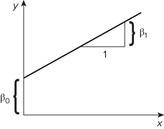

$\beta_{0}$ is an intercept when $\mathbf{X} = \mathbf{0}$.
$\beta_{1}$ is a slope that describes a change in average value for $y$ for each one-unit increase in $x_{1}$.
$\epsilon_{i}$ is the random noise.
- For inference, we need to assume that $\epsilon_{i}$ is independent, identically distributed (iid) from Normal distribution.

\[ \epsilon_i \overset{iid}{\sim}N(0, \sigma^2) \quad \text{ with constant variance } \sigma^2 \]

knitr::include_graphics('https://bcdanl.github.io/lec_figs/mba-1-3.png')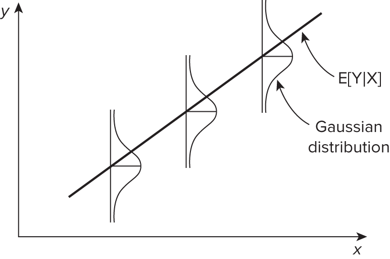

Fitted Line and Beta Estimates

We estimatede the best fitting line by ordinary least squares (OLS) - by minimizing the sum of squared errors (SSE)

\[ S S E\left(\beta_{0}, \beta_{1}\right)=\sum_{i=1}^{n}\left[Y_{i}-\left({\beta}_{0}+{\beta}_{1} X_{i}\right)\right]^{2} \]

knitr::include_graphics('https://bcdanl.github.io/lec_figs/mba-1-9.png')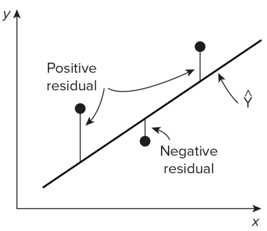

Therefore, the beta estimate has the following solution:

\[ \widehat{\beta}_{1}=\frac{\sum_{i=1}^{n}\left(X_{i}-\bar{X}\right)\left(Y_{i}-\bar{Y}\right)}{\sum_{i=1}^{n}\left(X_{i}-\bar{X}\right)^{2}} \quad \text{ and } \quad \widehat{\beta}_{0}=\bar{Y}-\widehat{\beta}_{1} \bar{X} \]

where $\bar{X} = \frac{1}{n}\sum_{i=1}^n X_i$ and $\bar{Y} = \frac{1}{n}\sum_{i=1}^n Y_i$

Connection to covariance and correlation

Covariance describes the joint variability of two variables

\[ \text{Cov}(X, Y) = \sigma_{X,Y} = \mathbb{E}[(X-\mathbb{E}[X])(Y-\mathbb{E}[Y])] \]

Correlation is a normalized form of covariance, ranges from -1 to 1

\[ \rho_{X,Y} = \frac{\text{Cov}(X,Y)}{\sigma_X \cdot \sigma_Y} \] - So, the beta coefficent can be represented by:

$$ \[\begin{align} \widehat{\beta}_{1} &= \, \frac{\widehat{\text{Cov}}(X,Y)}{\widehat{\text{Var}}(X)} \,=\, \hat{\rho}_{x,y} \cdot \frac{\hat{\sigma}_{Y}}{\hat{\sigma}_{X}} \end{align}\] $$

Inference with OLS

$t$-statistics are coefficients Estimates / Std. Error, i.e., number of standard deviations from 0
- p-values (i.e., Pr(>|t|)): estimated probability observing value as extreme as |t value| given the null hypothesis $\beta = 0$
- p-value $<$ conventional threshold of $\alpha = 0.05$, sufficient evidence to reject the null hypothesis that the coefficient is zero,
- Typically |t values| $> 2$ indicate significant relationship at $\alpha = 0.05$
- i.e., there is a significant association between log(sales) and log(price)
Controlling the Type 1 error rate at $\alpha = 0.05$, i.e., the probability of a false positive mistake:
- 5% chance that you’ll conclude there’s a significant association between $x$ and $y$ even when there is none

R-squared

$R^2$ estimates the proportion of the variance of $Y$ explained by $X$.

Mean Squared Errors

Mean squared error (MSE) is a commonly used metric to evaluate the performance of a regression model.
- It measures the average squared difference between the predicted values and the actual values in the dataset.

\[ M S E \,=\, \frac{\sum_{i = 1}^{ n}\,(\, y_{i} - \hat{y}_{i} \,)^2}{n} \] - Root mean squared error (RMSE) is the square root of the mean squared error (MSE).

\[ R M S E \,=\, \sqrt{M S E} \] - RMSE shows how far predictions fall from true values.

The Goals of Linear Regression

Modeling for prediction ($\hat{y}$): When we want to predict an outcome variable $y$ based on the information contained in a set of predictor variables $\mathbf{X}$.

We are estimating the conditional expection (mean) for $y$: \[ \mathbb{E}[\, y \,|\, \mathbf{X} \,] = \beta_{0} \,+\, \beta_{1}\,x_{1} \,+\, \cdots \,+\, \beta_{p}\,x_{p}. \]
which is the average value for $y$ given the value for $X$.

Modeling for explanation ($\hat{\beta}$): When we want to explicitly describe and quantify the relationship between the outcome variable $y$ and a set of explanatory variables $\mathbf{X}$.

Correlation does not imply causation.
Without proper identification strategies, $\beta_{1}$ just means a correlation between $x_{1}$ and $y$.
However, we can possibly identify a causal relationship between the explanatory variable and the outcome variable.

Linear Regression and Controls

Simple Linear Regression

To start, we can fit a simple model that regresses log price on log sales.

\[ \mathbb{E}[\, \log(\, \texttt{sales} \,) \,|\, \texttt{price}\,] = \alpha \,+\, \beta\, \log(\,\texttt{price}\,) \] - The following model incorporates both brand and price:

\[ \mathbb{E}[\, \log(\, \texttt{sales} \,) \,|\, \texttt{price}\,] = \alpha_{\texttt{brand}} \,+\, \beta\, \log(\,\texttt{price}\,) \]

formula_0 <- log(sales) ~ log(price)
formula_1 <- log(sales) ~ brand + log(price)

fit_0 <- lm( formula_0, data = oj )
fit_1 <- lm( formula_1, data = oj )

stargazer(fit_0, fit_1, type = "html")


	Dependent variable:

	log(sales)
	(1)	(2)

brandminute.maid		0.870^***
		(0.013)

brandtropicana		1.530^***
		(0.016)

log(price)	-1.601^***	-3.139^***
	(0.018)	(0.023)

Constant	10.423^***	10.829^***
	(0.015)	(0.015)


Observations	28,947	28,947
R²	0.208	0.394
Adjusted R²	0.208	0.394
Residual Std. Error	0.907 (df = 28945)	0.794 (df = 28943)
F Statistic	7,608.212^*** (df = 1; 28945)	6,275.074^*** (df = 3; 28943)

Note:	p<0.1; p<0.05; p<0.01

We know that there are different brands of OJ here and some are more valuable than others.
- When we control for brand effect, the elasticity estimate nearly doubles to −3.14.
The premium brands, Minute Maid and Tropicana, had equivalent sales to Dominick’s at higher price points.
So if we don’t control for brand, it looks as though prices can rise without affecting sales for those observations.
- This dampens the observable relationship between prices and sales and results in the (artificially) low elasticity estimate of −1.6.
More mechanically, how does this happen in regression?

price_fit <- lm(log(price) ~ brand, data = oj)
p_hat <- predict(price_fit, newdata = oj)
p_resid <- log(oj$price) - p_hat

# regress log sales on p_resid
resid_fit <- lm(log(sales) ~ p_resid, data = oj)

# What is the beta coefficient for p_resid?!
round( coef(resid_fit)[2], digit = 3 )

p_resid 
 -3.139

The coefficient on p_resid, the residuals from regression of log price on brand, is exactly the same as what we get on log(price) in the multiple linear regression for log sales onto this and brand!
This is one way that you can understand what OLS is doing:
- It is finding the coefficients on the part of each input that is independent from the other inputs.

Controls in Linear Regression

Omitted variable bias is a type of bias that can occur in linear regression when an important variable that is related to both the outcome variable and the input variable(s) is not included in the model.
- This omission can lead to biased estimates of the beta coefficients of the included input variables.
In linear regression, a confounding variable is a variable that is related to both treatment and outcome variables, and that affects the relationship between them.
- A treatment variable is an input variable that the researcher believes has a causal effect on the outcome variable.
- When a confounding variable is not controlled in the regression model, it can lead to biased estimates of the relationship between the independent and treatment variables.
Bad controls in linear regression refer to the inclusion of variables in the model that do not actually control for the confounding factors they are intended to control for.
- This can lead to biased estimates of the relationship between the independent and dependent variables.

# simulation data
tb <- tibble( 
  female = ifelse(runif(10000)>=0.5,1,0), # female indicator variable
  ability = rnorm(10000), # e.g., talent, usually unobserved.
  discrimination = female, # gender discrimination variable
  occupation = 1 + 2*ability + 0*female - 2*discrimination + rnorm(10000), # true data generating process for occupation variable
  wage = 1 - 1*discrimination + 1*occupation + 2*ability + rnorm(10000) # true data generating process for wage variable
)

lm_1 <- lm(wage ~ female, tb)
lm_2 <- lm(wage ~ female + occupation, tb)
lm_3 <- lm(wage ~ female + occupation + ability, tb)

stargazer(lm_1,lm_2,lm_3, 
          column.labels = c("Biased Unconditional", 
                            "Biased",
                            "Unbiased Conditional"),
          type = 'html')


	Dependent variable:

	wage
	Biased Unconditional	Biased	Unbiased Conditional
	(1)	(2)	(3)

female	-3.012^***	0.622^***	-0.991^***
	(0.085)	(0.030)	(0.028)

occupation		1.804^***	0.993^***
		(0.006)	(0.010)

ability			2.026^***
			(0.022)

Constant	1.952^***	0.207^***	1.005^***
	(0.060)	(0.020)	(0.017)


Observations	10,000	10,000	10,000
R²	0.112	0.909	0.950
Adjusted R²	0.112	0.909	0.950
Residual Std. Error	4.237 (df = 9998)	1.355 (df = 9997)	1.004 (df = 9996)
F Statistic	1,263.492^*** (df = 1; 9998)	50,026.950^*** (df = 2; 9997)	63,578.110^*** (df = 3; 9996)

Note:	p<0.1; p<0.05; p<0.01

occupation is a bad control.

Residual plot, QQ plot, and Residual vs Leverage plot

Residuals should NOT display any systematic pattern.
Check the assumptions about normality with a QQ plot using ggfortify.

library(ggfortify)
autoplot(fit_1, ncol = 1)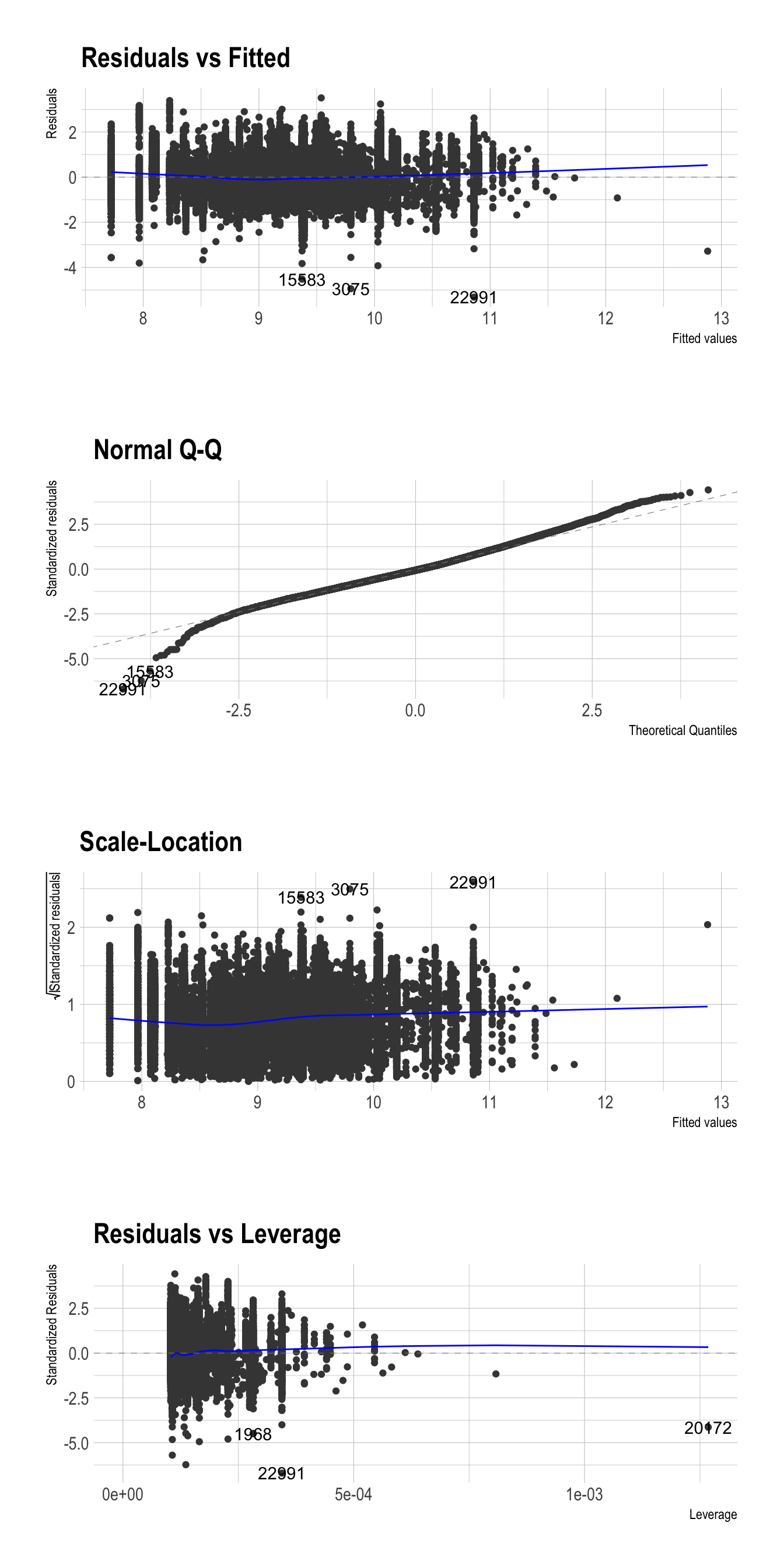

Standardized residuals = residuals / sd(residuals)
A QQ (Quantile-Quantile) plot is a graphical tool used to assess the normality of a distribution.
- In the context of linear regression, a QQ plot can be used to assess whether the residuals are normally distributed.
- A QQ plot visualizes the relationship between the quantiles of the residuals and the quantiles of a theoretical normal distribution.
- QQ plots can be useful in identifying potential outliers or influential observations in a linear regression model, as well as in deciding whether to transform the dependent variable or use a different type of regression model altogether.
A residual vs leverage plot is a graphical tool used to detect influential observations in linear regression.
- Leverage refers to how much an observation’s independent variables differ from the mean of the independent variables, and is a measure of how much influence that observation has on the regression line.
- In a residual vs leverage plot, influential observations will typically appear as points that are far away from the center of the plot.
- If an observation has high leverage but a small residual, it may not be influential.
- Conversely, an observation with a large residual but low leverage may also not be influential.

Fixed effects

Unobserved characteristics that is associated with at least one explanatory variable is called a “fixed effect”.
If there exists the fixed effect in the data and we do not control the fixed effect in the model, the model will have a biased result in estimation.
We often control unobserved characteristics across countries/individuals/firms/counties/US states by including dummy variables of those entities in the model.
- For example, some unobserved characteristics across countries in the world (like governance effectiveness, investment in electricity grid, etc.) is likely to be associated with variable of access to electricity.
- If such unobserved characteristics are not controlled in the model, the model result will be likely to be biased.
- This is because one of the most crucial assumptions in regression—errors are not correlated with explanatory variables $E[\,\epsilon_{i} | X\,] \,=\, 0$—is not likely to hold without controlling such unobserved characteristics.
- The following is the OLS estimator $\hat{\beta}$ for the true beta $\beta$ in a matrix form.

\[\begin{align} \hat{\beta} \,=\,& \beta + E[\,(X'X)^{-1}X'\epsilon\,]\\ \,\neq\,& \beta \qquad \text{ if } E[\,\epsilon_{i} | X\,] \,\neq\, 0\end{align}\]
- Without controlling such unobserved characteristics, the beta estimator cannot be the same as the true beta at all.

Exercise

Consider the orange juice models:

formula_0 <- log(sales) ~ log(price)
formula_1 <- log(sales) ~ brand + log(price)

fit_0 <- lm( formula_0, data = oj )
fit_1 <- lm( formula_1, data = oj )

Draw a residual plot for each model of fit_0 and fit_1.
Calculate the RMSE for each model of fit_0 and fit_1.
Review the interaction models:

formula_0 <- log(sales) ~ log(price)
formula_1 <- log(sales) ~ brand + log(price)
formula_2 <- log(sales) ~ brand * log(price)
formula_3 <- log(sales) ~ brand * ad * log(price)

fit_0 <- lm( formula_0, data = oj )
fit_1 <- lm( formula_1, data = oj )
fit_2 <- lm( formula_2, data = oj )
fit_3 <- lm( formula_3, data = oj )

stargazer(fit_1, fit_2, fit_3, type = "html")


	Dependent variable:

	log(sales)
	(1)	(2)	(3)

brandminute.maid	0.870^***	0.888^***	0.047
	(0.013)	(0.042)	(0.047)

brandtropicana	1.530^***	0.962^***	0.708^***
	(0.016)	(0.046)	(0.051)

ad			1.094^***
			(0.038)

log(price)	-3.139^***	-3.378^***	-2.774^***
	(0.023)	(0.036)	(0.039)

brandminute.maid:ad			1.173^***
			(0.082)

brandtropicana:ad			0.785^***
			(0.099)

brandminute.maid:log(price)		0.057	0.783^***
		(0.057)	(0.061)

brandtropicana:log(price)		0.666^***	0.736^***
		(0.054)	(0.057)

ad:log(price)			-0.471^***
			(0.074)

brandminute.maid:ad:log(price)			-1.109^***
			(0.122)

brandtropicana:ad:log(price)			-0.986^***
			(0.124)

Constant	10.829^***	10.955^***	10.407^***
	(0.015)	(0.021)	(0.023)


Observations	28,947	28,947	28,947
R²	0.394	0.398	0.535
Adjusted R²	0.394	0.398	0.535
Residual Std. Error	0.794 (df = 28943)	0.791 (df = 28941)	0.695 (df = 28935)
F Statistic	6,275.074^*** (df = 3; 28943)	3,823.404^*** (df = 5; 28941)	3,031.232^*** (df = 11; 28935)

Note:	p<0.1; p<0.05; p<0.01

References

Modern Business Analytics by Matt Taddy, Leslie Hendrix, and Matthew Harding.

Summer Undergraduate Research Experience (SURE) 2022 in Statistics at Carnegie Mellon University by Ron Yurko.