Lecture 3
Logistic Regression
February 11, 2026
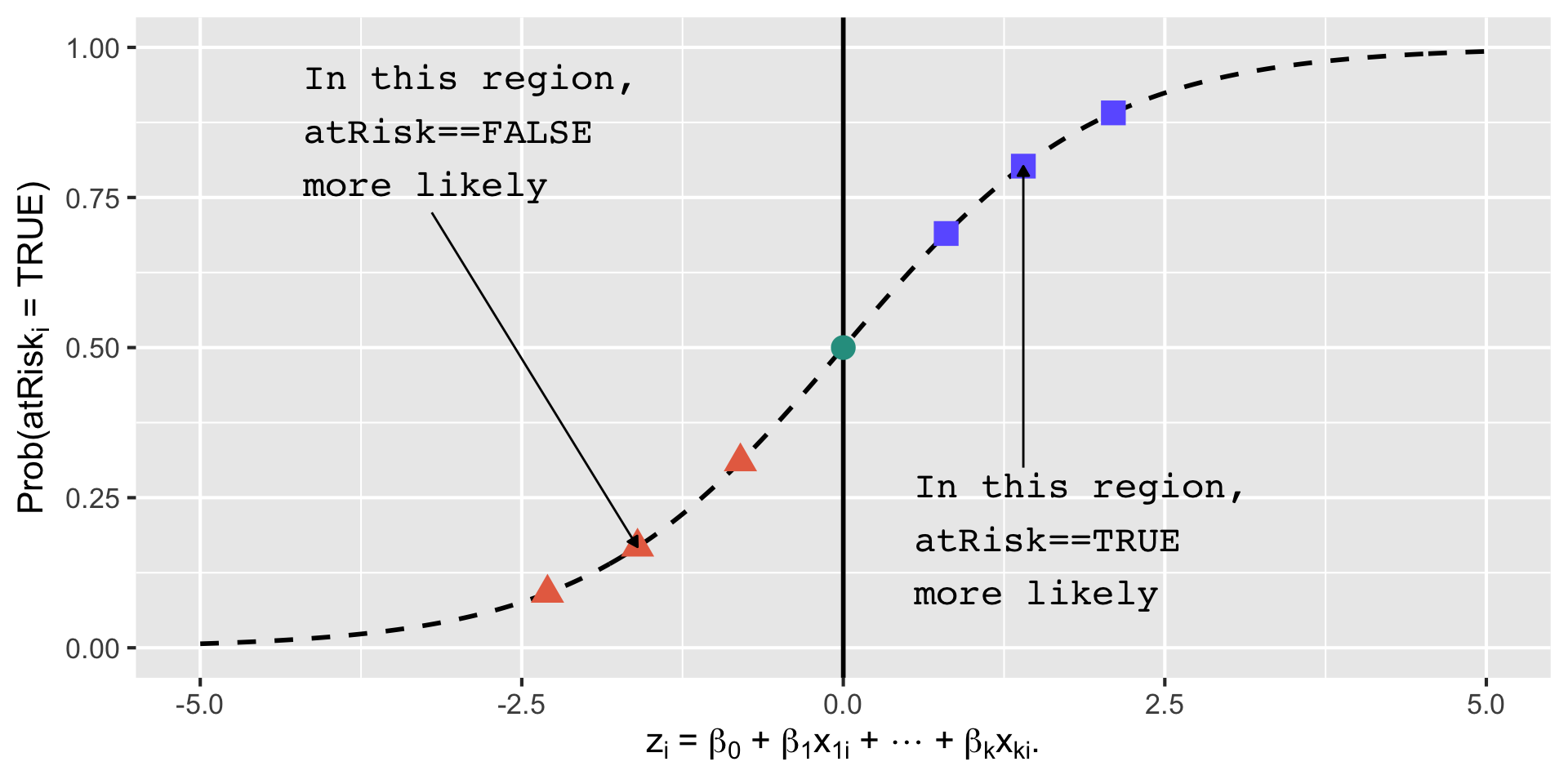
Logistic Function
Likelihood Function
- Likelihood is the probability of your data given the model.
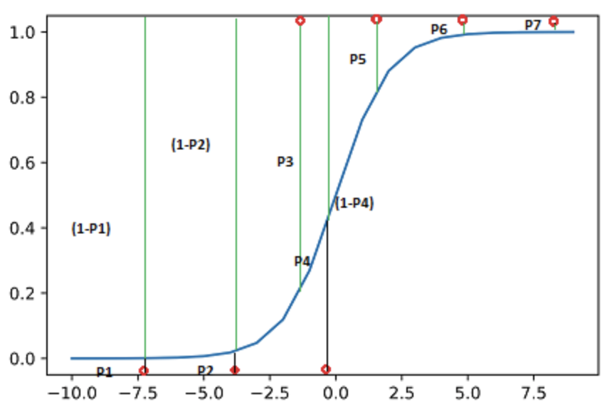
- The probability that the seven data points would be observed:
- \(L = (1-P1)\times(1-P2)\times P3 \times (1-P4) \times P5 \times P6 \times P7\)
- The log of the likelihood: \[ \begin{align} \log(L) &= \log(1-P1) + \log(1-P2) + \log(P3) \\ &\quad+ \log(1-P4) + \log(P5) + \log(P6) + \log(P7) \end{align} \]
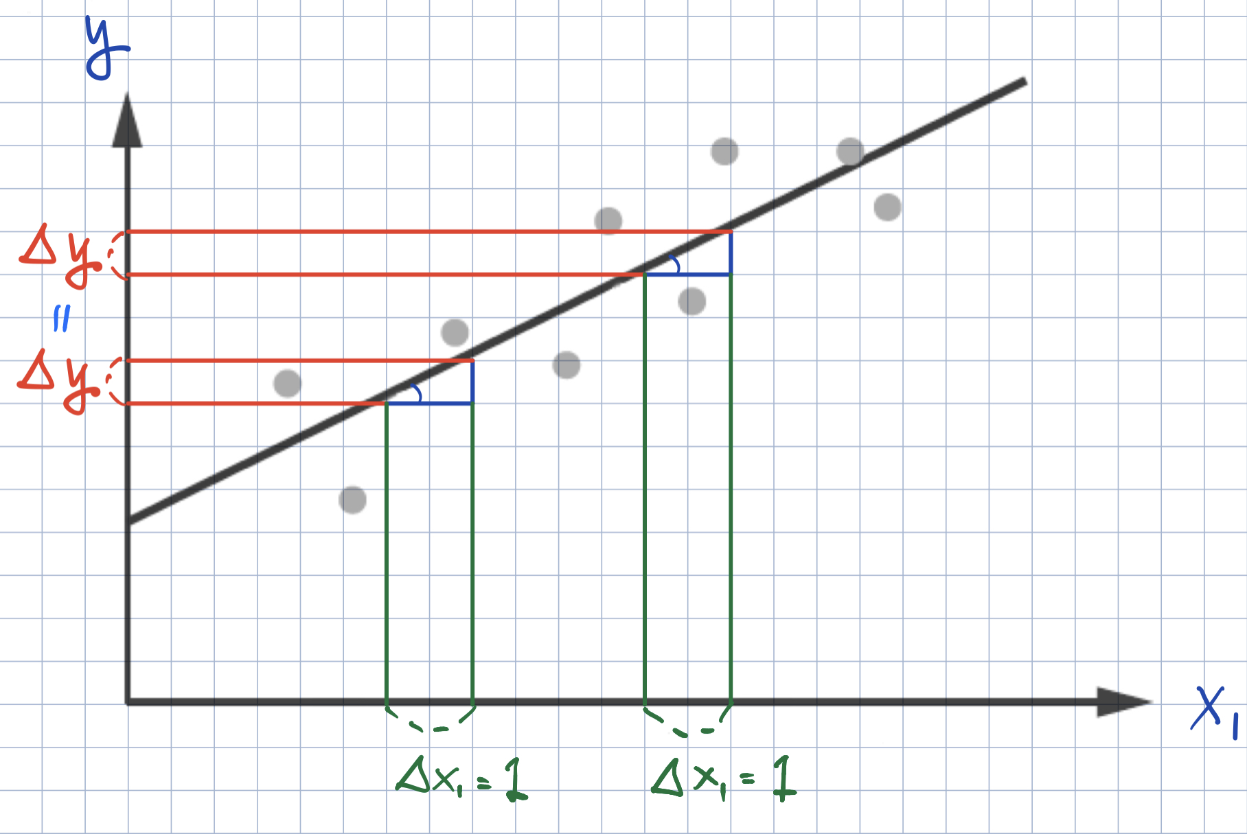
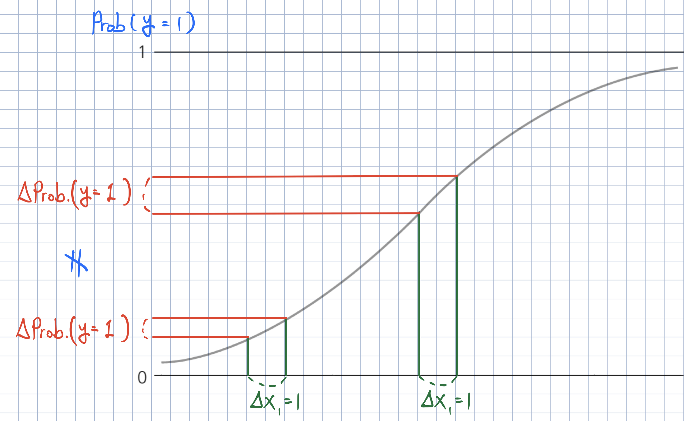
Marginal Effect of \(x_{k, i}\) on \(\text{Prob}(y_{i} = 1)\)
- In logistic regression, the effect of \(x_{k, i}\) on \(\text{Prob}(y_{i} = 1)\) is different for each observation \(i\).
Accuracy
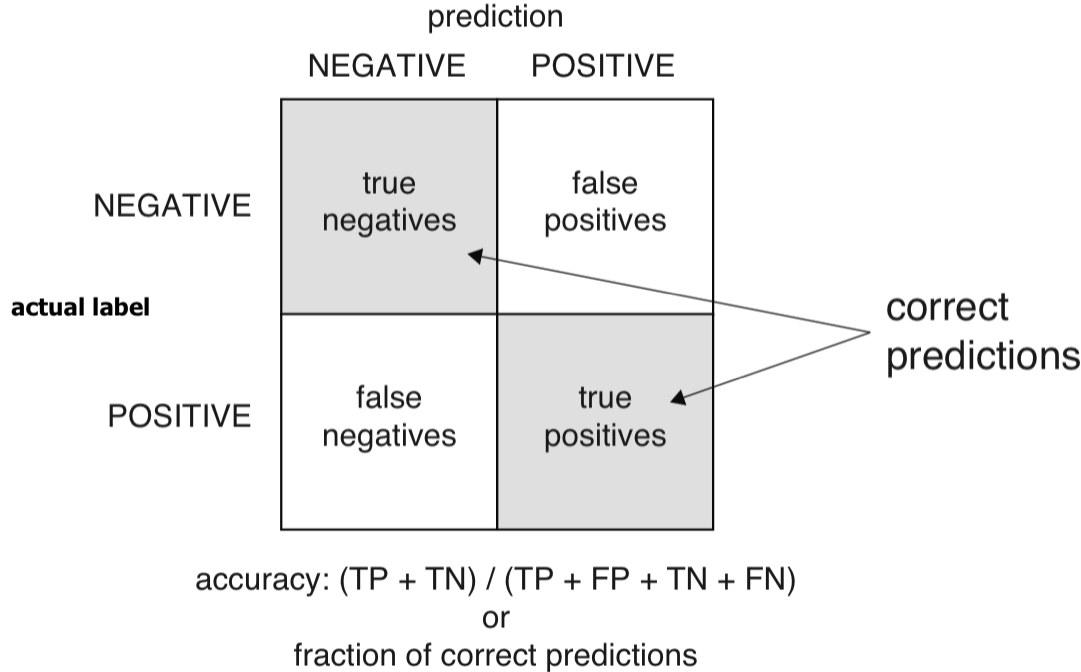
- Accuracy: When the classifier says this newborn baby is at risk or is not at risk, what is the probability that the model is correct?
- Accuracy is defined as the number of items categorized correctly divided by the total number of items.
Precision
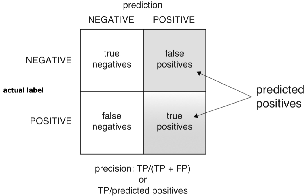
- Precision: If the classifier says this newborn baby is at risk, what’s the probability that the baby is really at risk?
- Precision is defined as the ratio of true positives to predicted positives.
Recall (or Sensitivity)
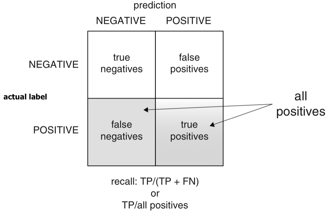
- Recall (or sensitivity): Of all the babies at risk, what fraction did the classifier detect?
- Recall (or sensitivity) is also called the true positive rate (TPR), the ratio of true positives over all actual positives.
Specificity
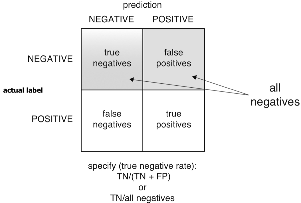
- Specificity: Of all the not-at-risk babies, what fraction did the classifier detect?
- Specificity is also called the true negative rate (TNR), the ratio of true negatives over all actual negatives.
ROC and AUC
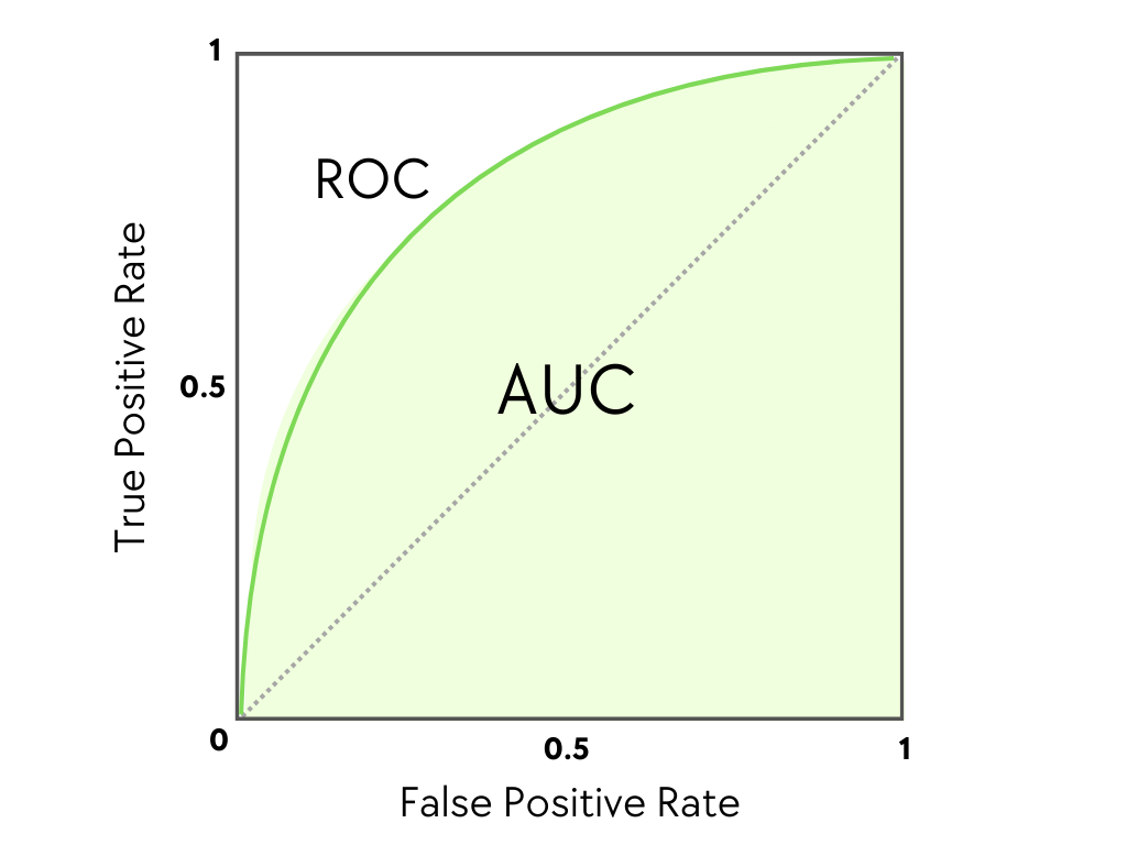
The receiver operating characteristic curve (or ROC curve) plots both the true positive rate (recall) and the false positive rate (or 1 - specificity) for all threshold levels.
- Area under the curve (or AUC) can be another measure of the quality of the model.
ROC - (0,0)
- (0,0)—Corresponding to a classifier defined by the threshold \(\text{Prob}(y_{i} = 1) = 1\):
- Nothing gets classified as at-risk.
ROC - (1,1)
- (1,1)—Corresponding to a classifier defined by the threshold \(\text{Prob}(y_{i} = 1) = 0\):
- Everything gets classified as at-risk.
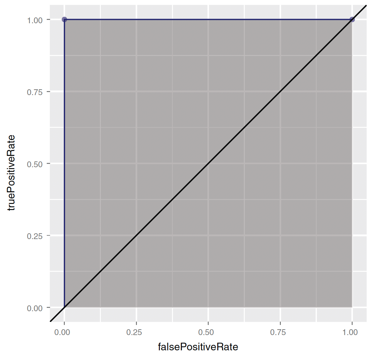
ROC - (0,1)
- (0,1)—Corresponding to any classifier defined by a threshold between 0 and 1:
- Everything is classified perfectly!
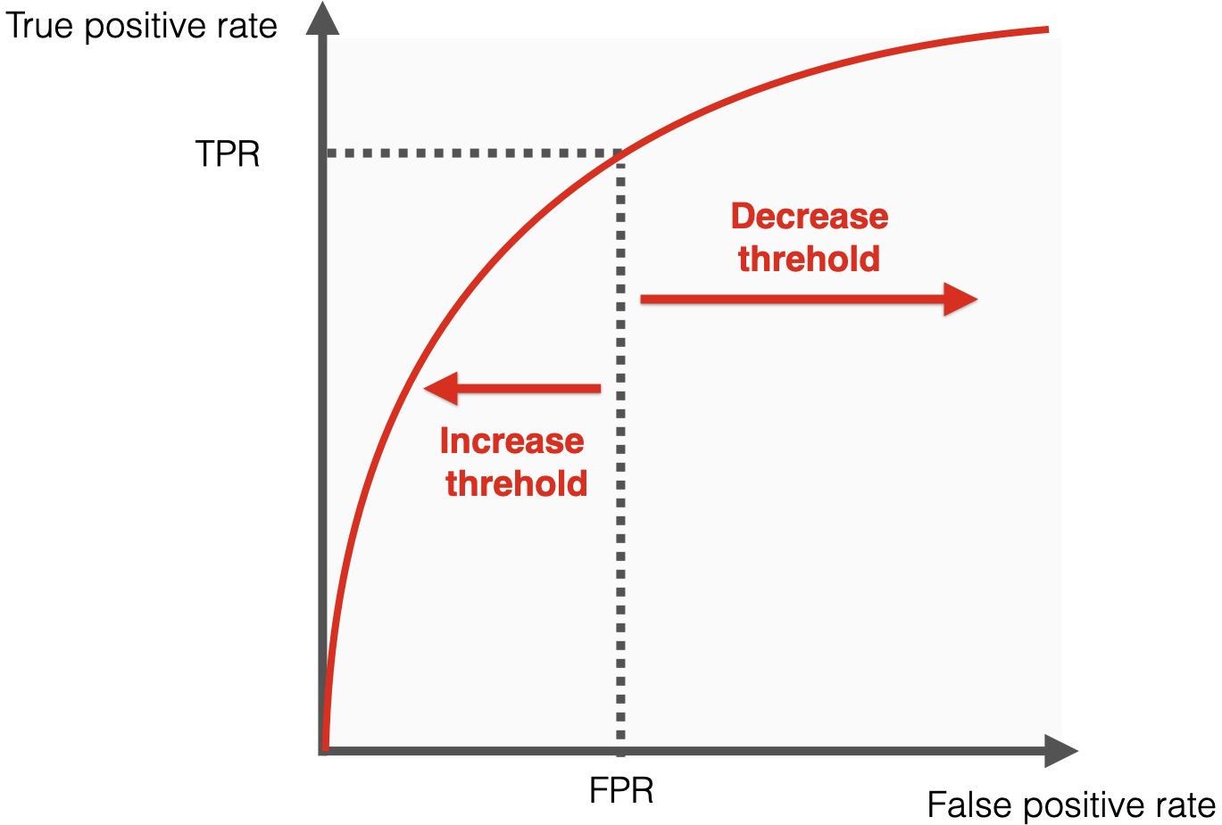
ROC and Thresholds
AUC
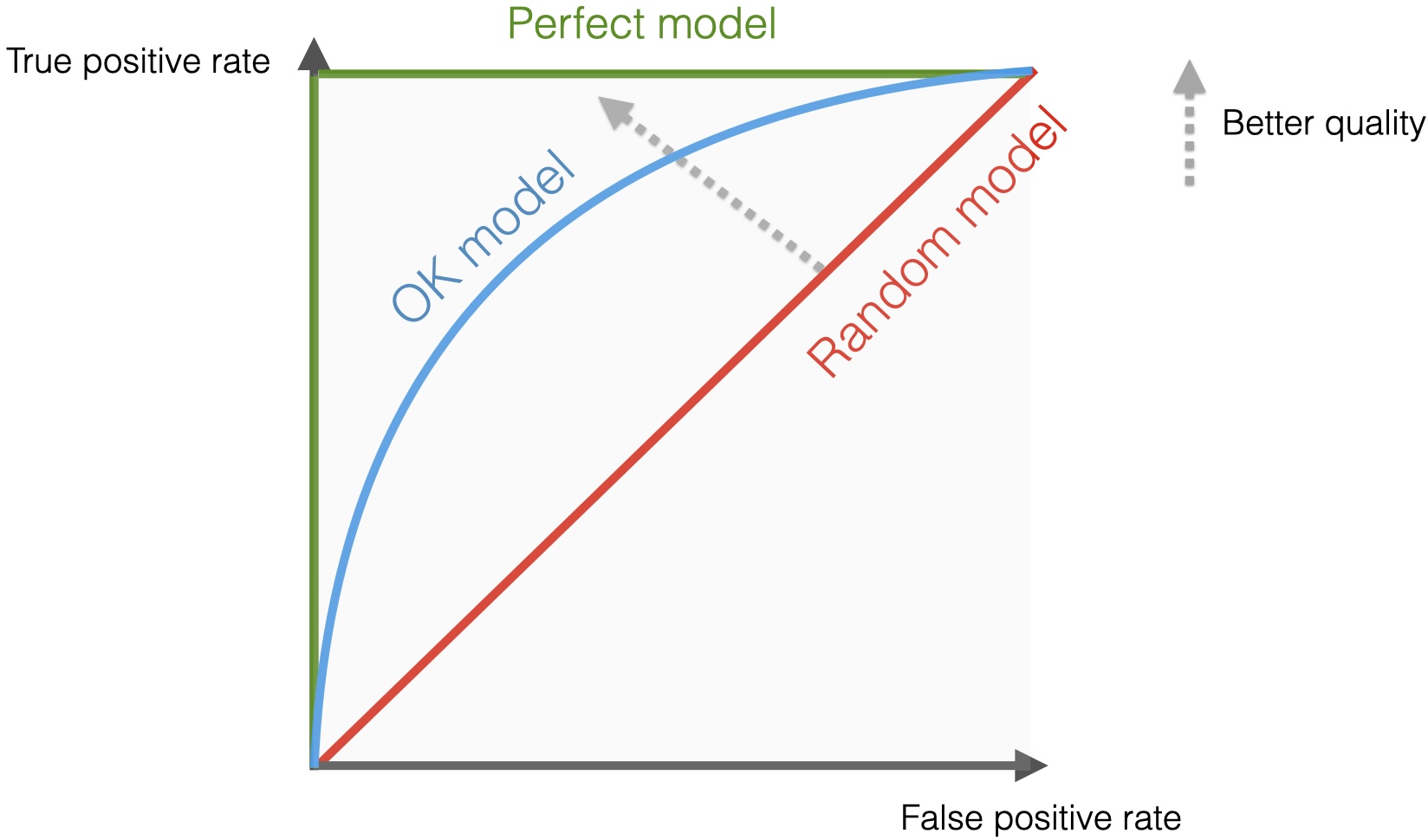
- AUC measures overall performance across all thresholds, with 1.0 being perfect.