Lecture 2
Data Visualization with ggplot
January 26, 2026
Grammar of Graphics
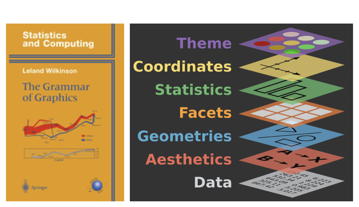
- A grammar of graphics is a tool that enables us to concisely describe the components of a graphic.
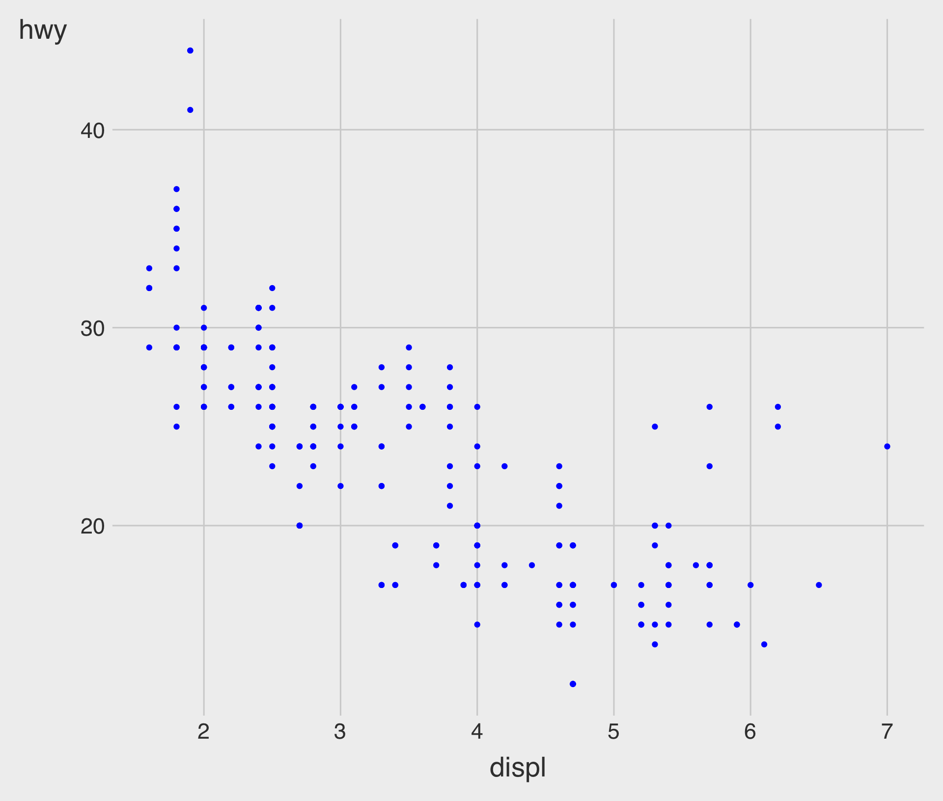
Creating a Scatterplot with ggplot
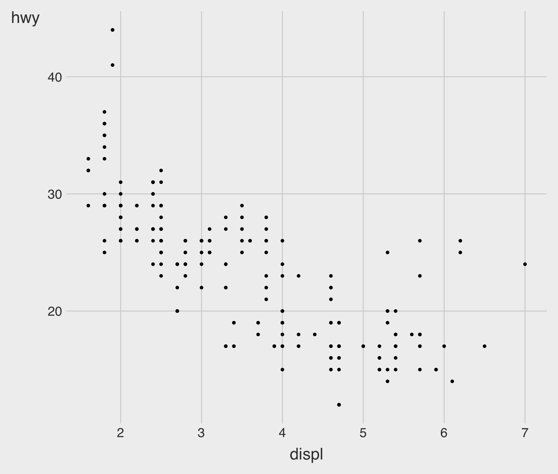
- To plot
mpg, run the above code to putdisplon thex-axis andhwyon they-axis.
Scatterplot with geom_point()

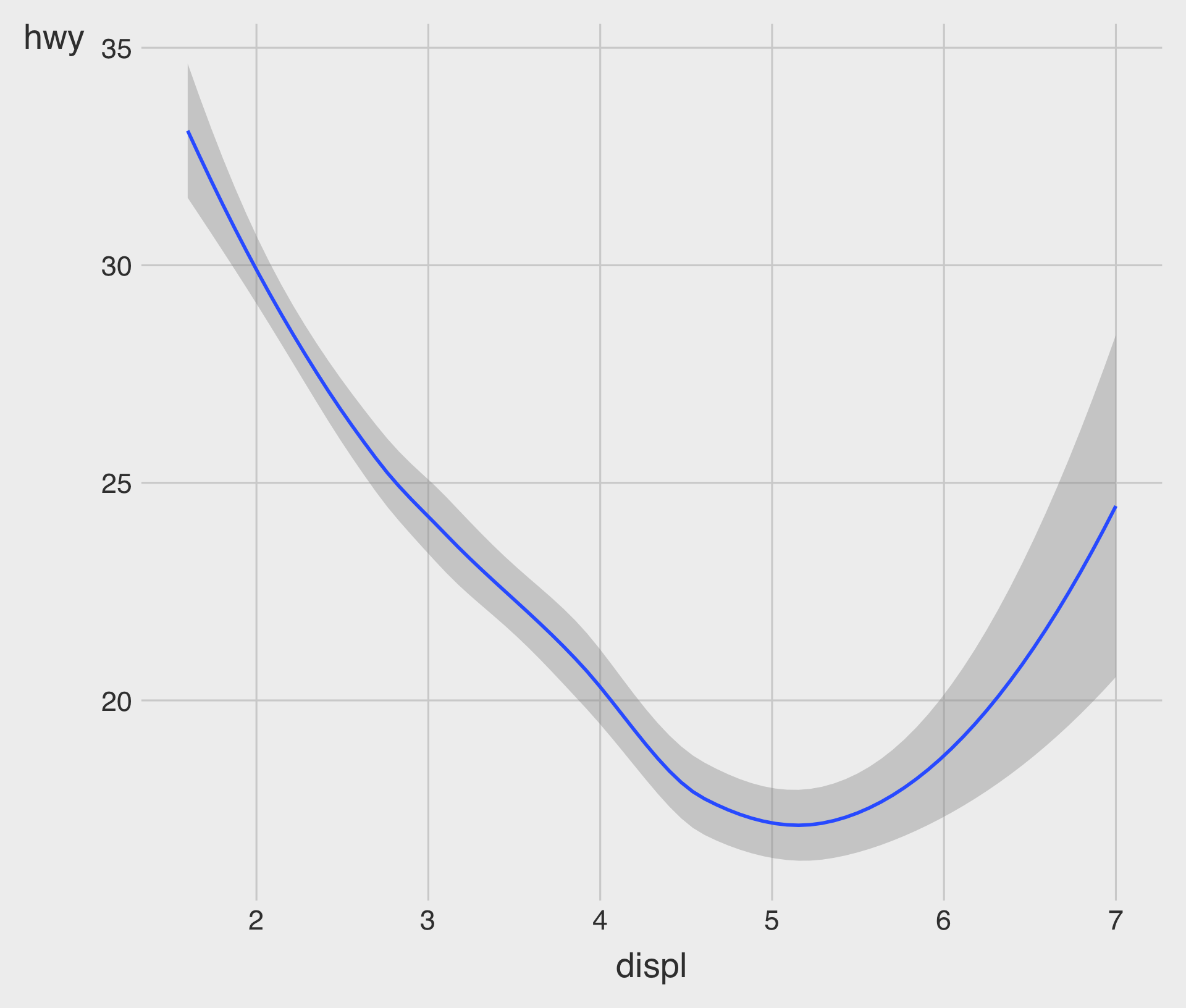
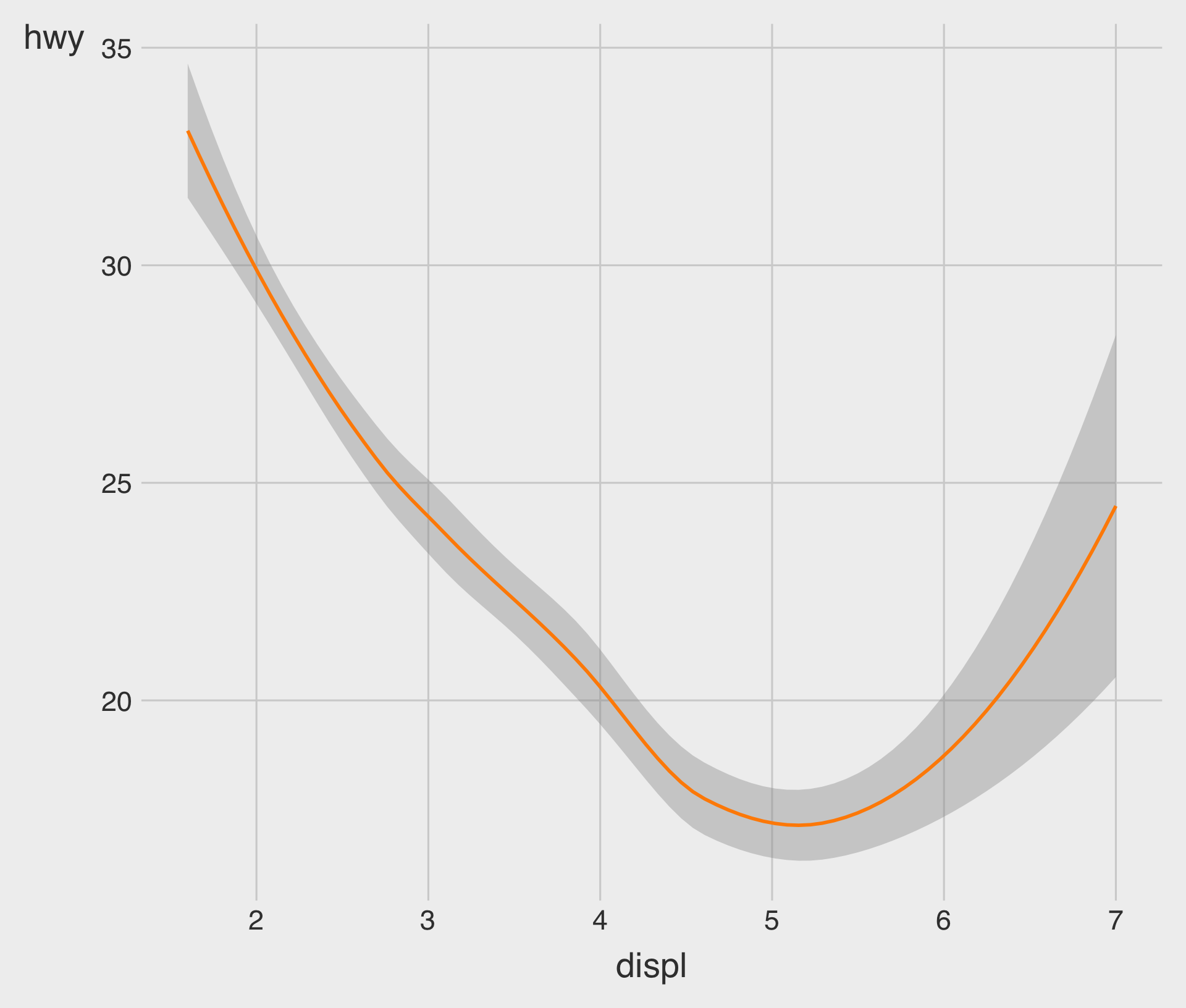
Fitted Curve with geom_smooth()
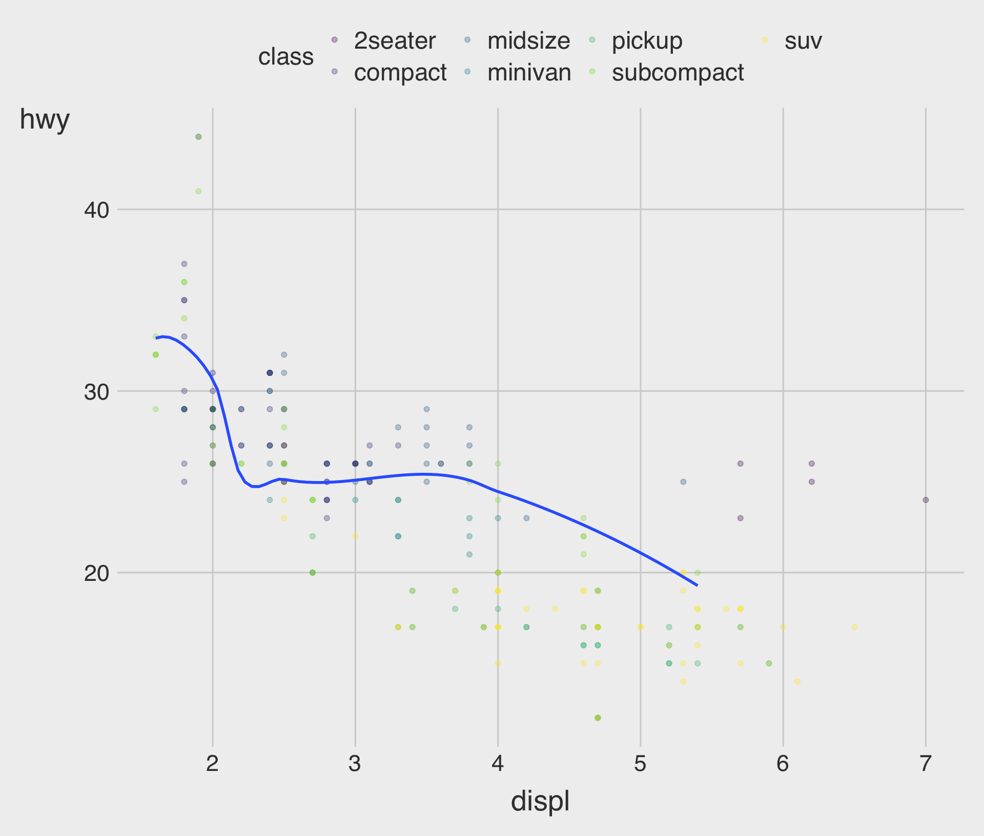
geom_point() with geom_smooth()
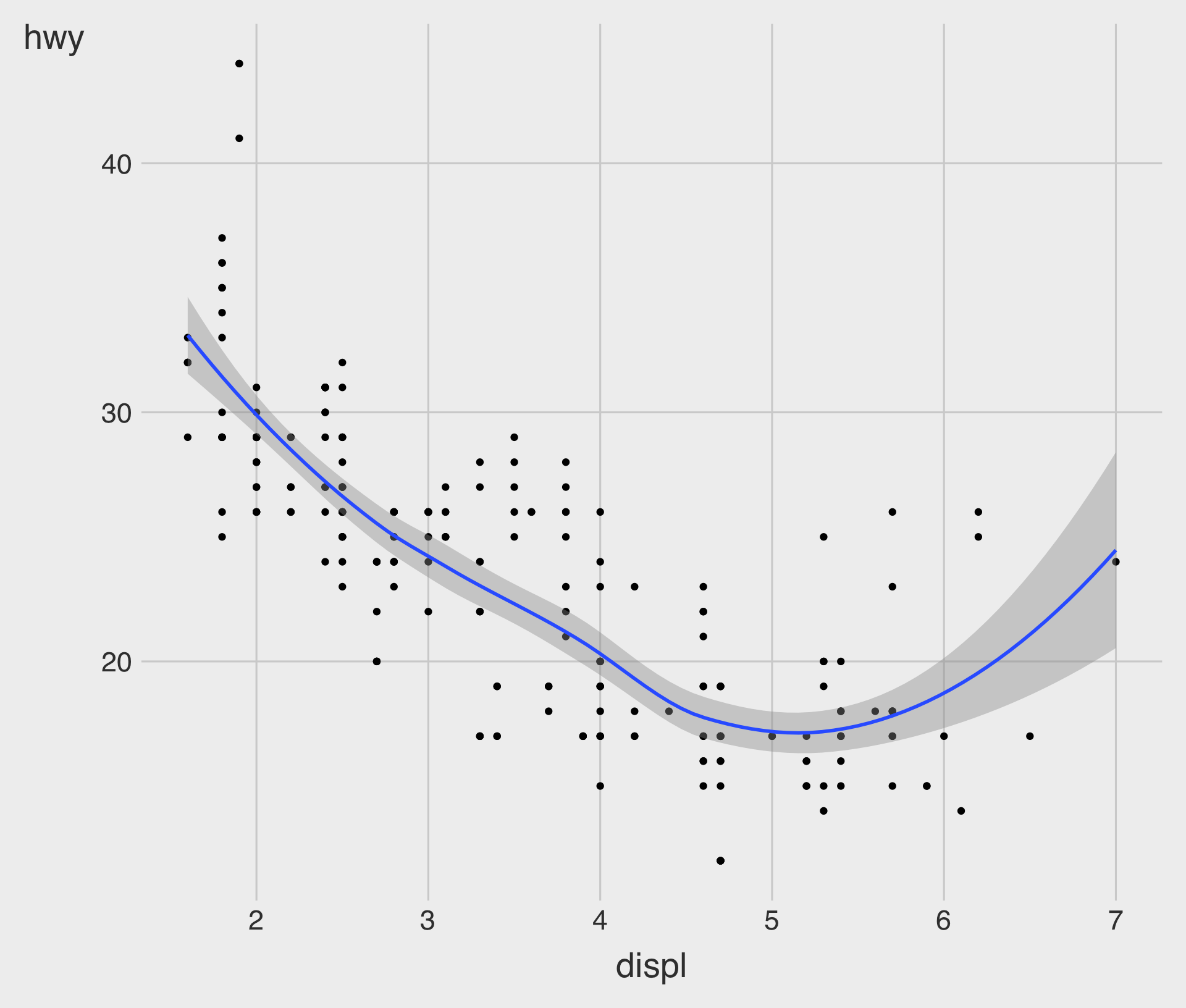
- The geometric object
geom_smooth()draws a smooth curve fitted to the data.
geom_point() with geom_smooth(method = lm)
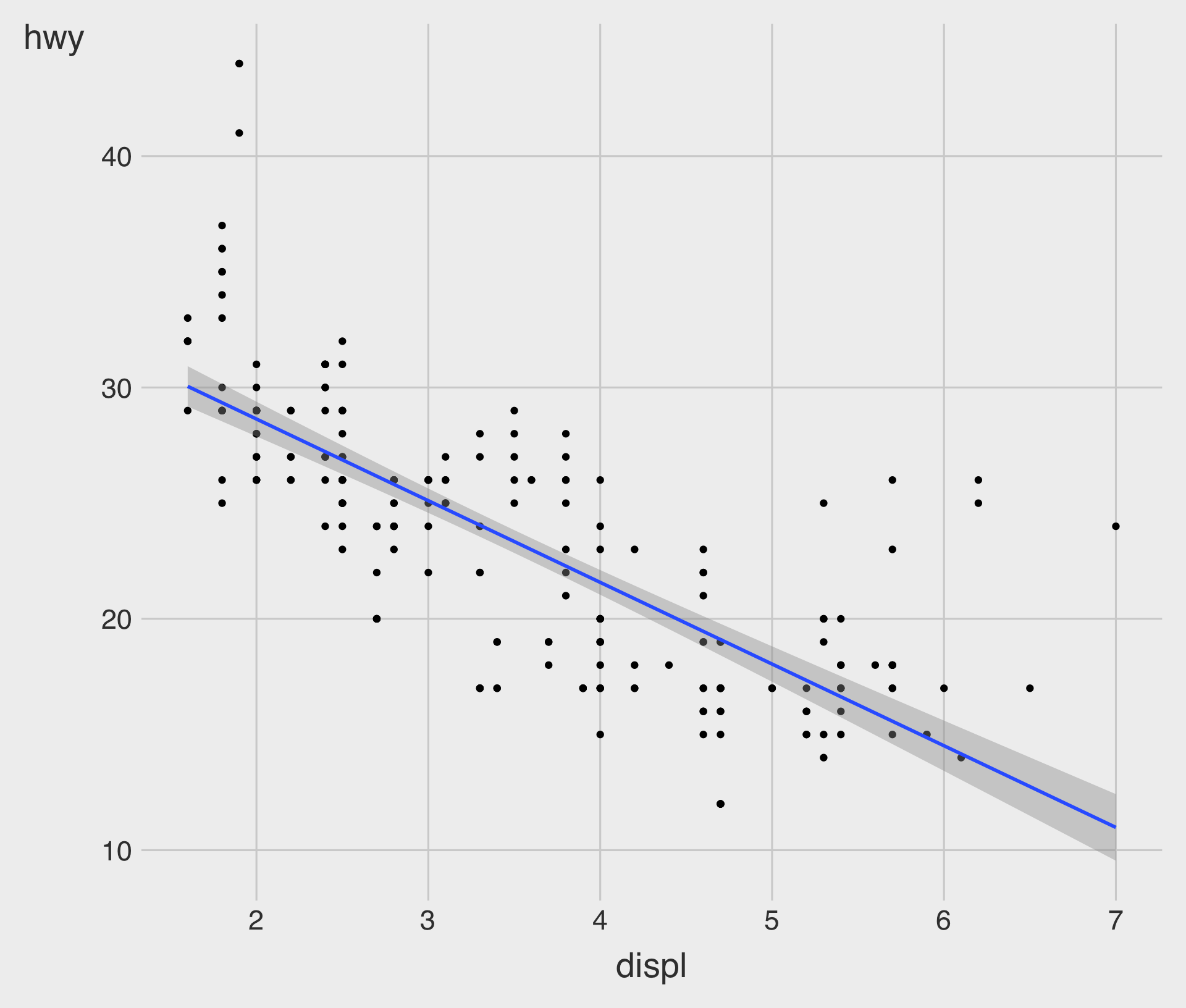
method = "lm"specifies that a linear model (lm), called a linear regression model.
Relationship ggplot()
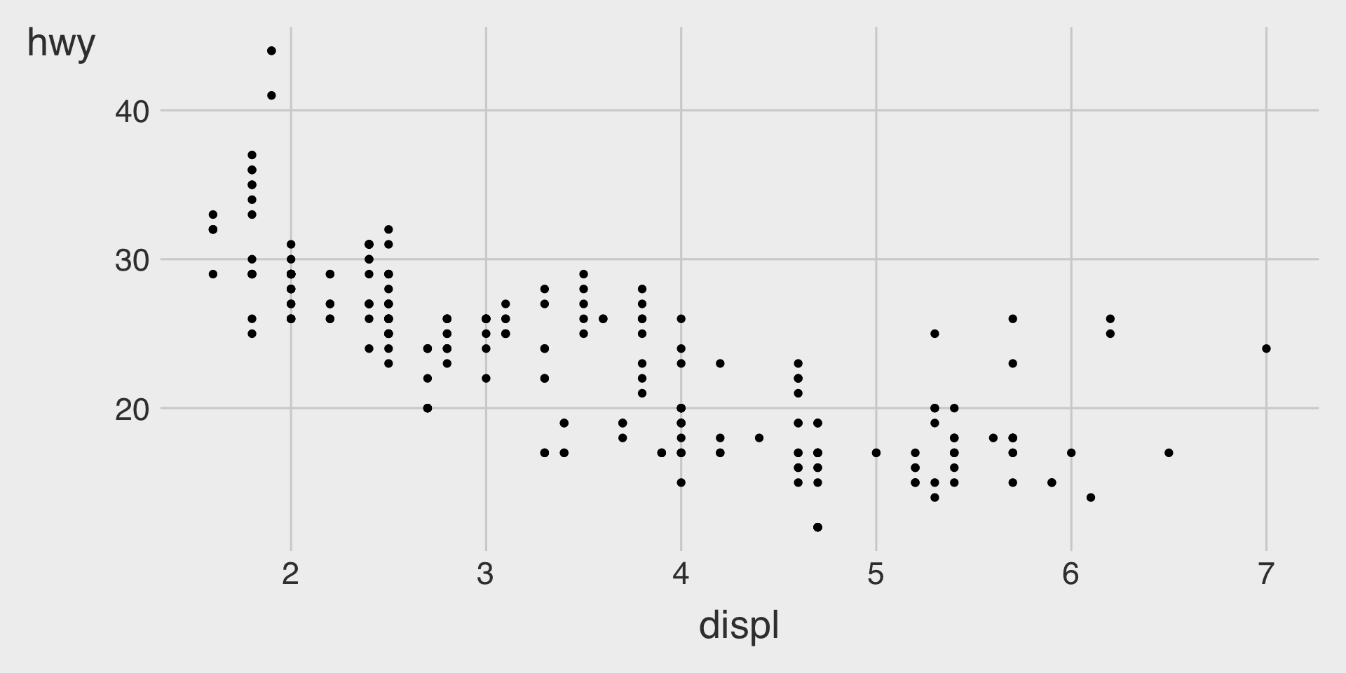
- How many points are in this plot?
- How many observations are in the
mpgdata.frame?
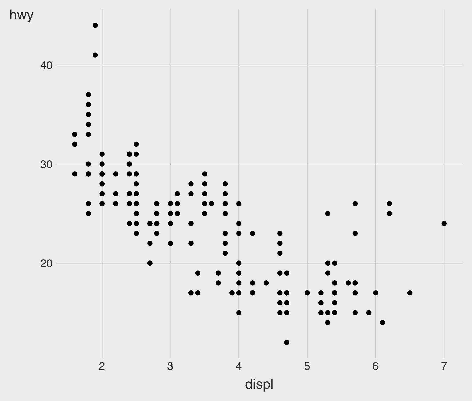
Overplotting and Transparency with alpha

- We can set a transparency level (
alpha) between 0 (full transparency) and 1 (no transparency) manually.
Overplotting and Transparency with alpha
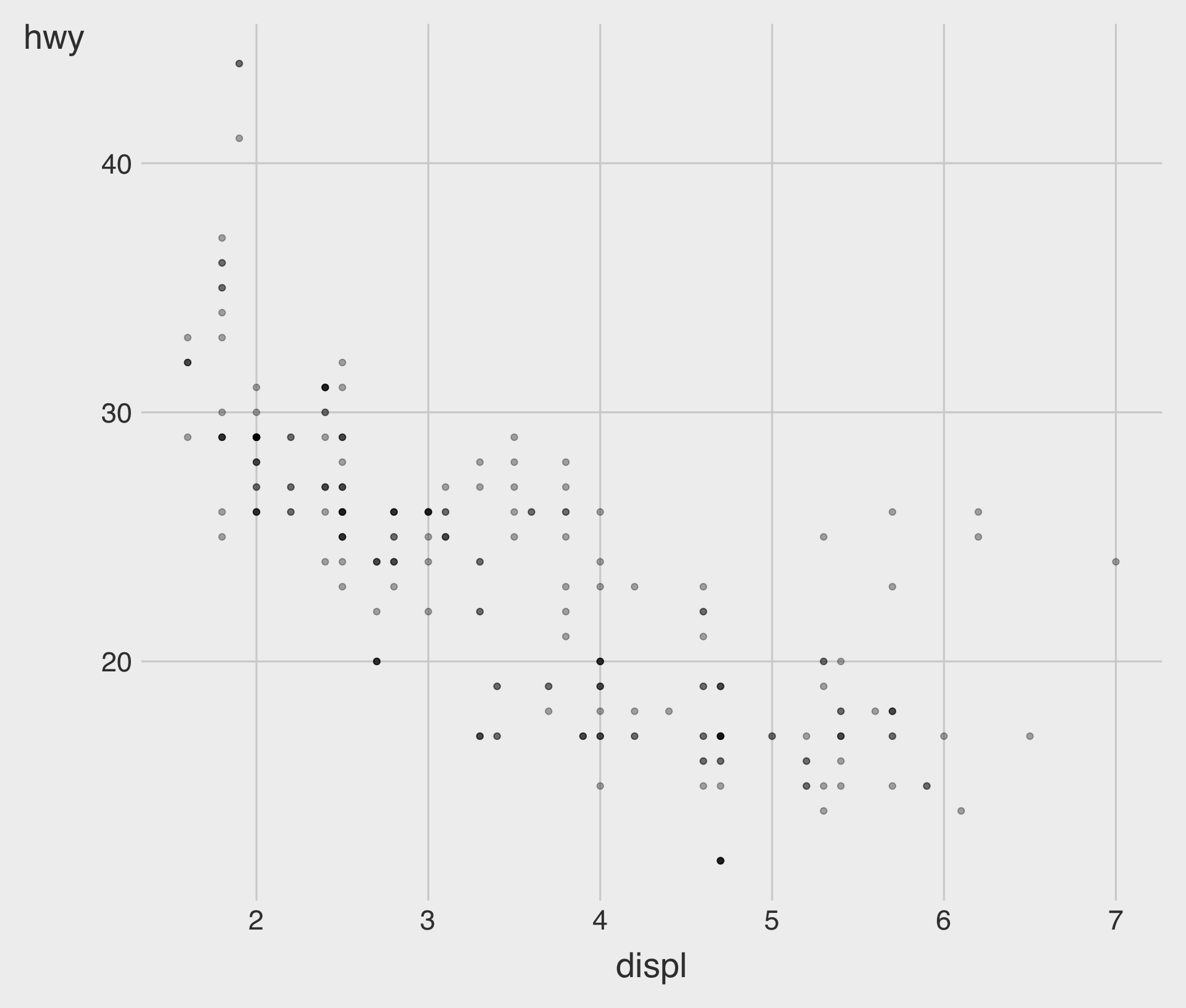
- We can set an aesthetic property manually, as seen above, not within the
aes()function but within thegeom_*()function.
Aesthetic Mappings
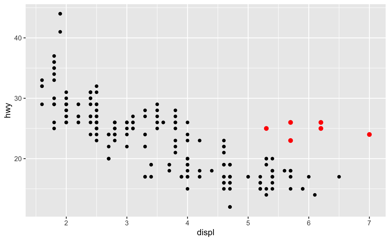
In the plot above, one group of points (highlighted in red) seems to fall outside of the linear trend.
- How can you explain these cars? Are those hybrids?
Aesthetic Mappings
An aesthetic is a visual property (e.g.,
size,shape,color) of the objects (e.g.,class) in your plot.You can display a point in different ways by changing the values of its aesthetic properties.
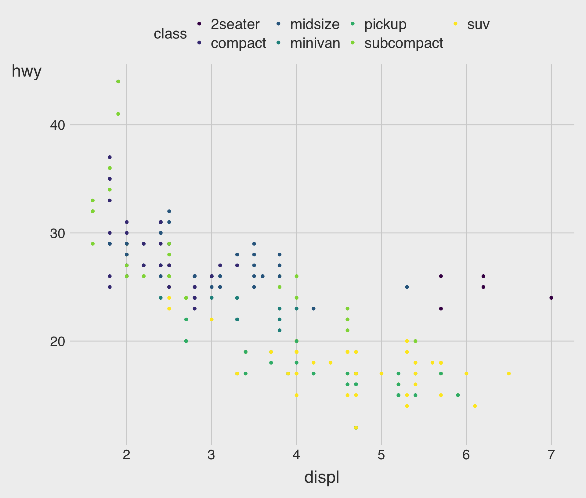
Adding a color to the Plot
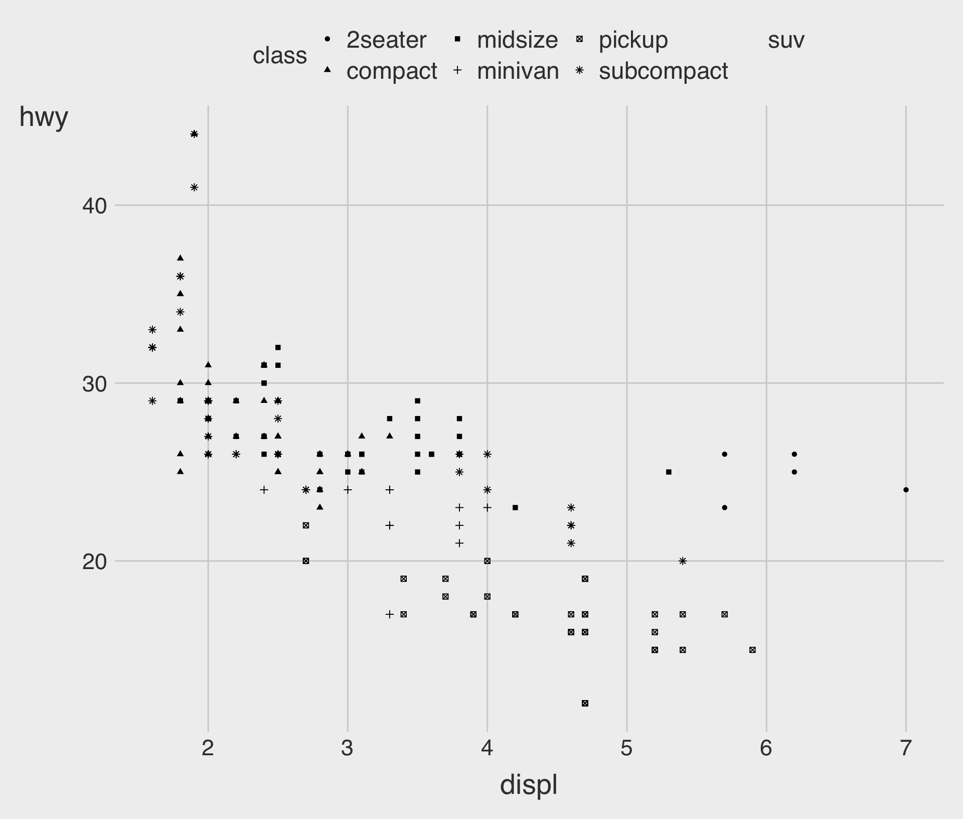
Adding a shape to the Plot
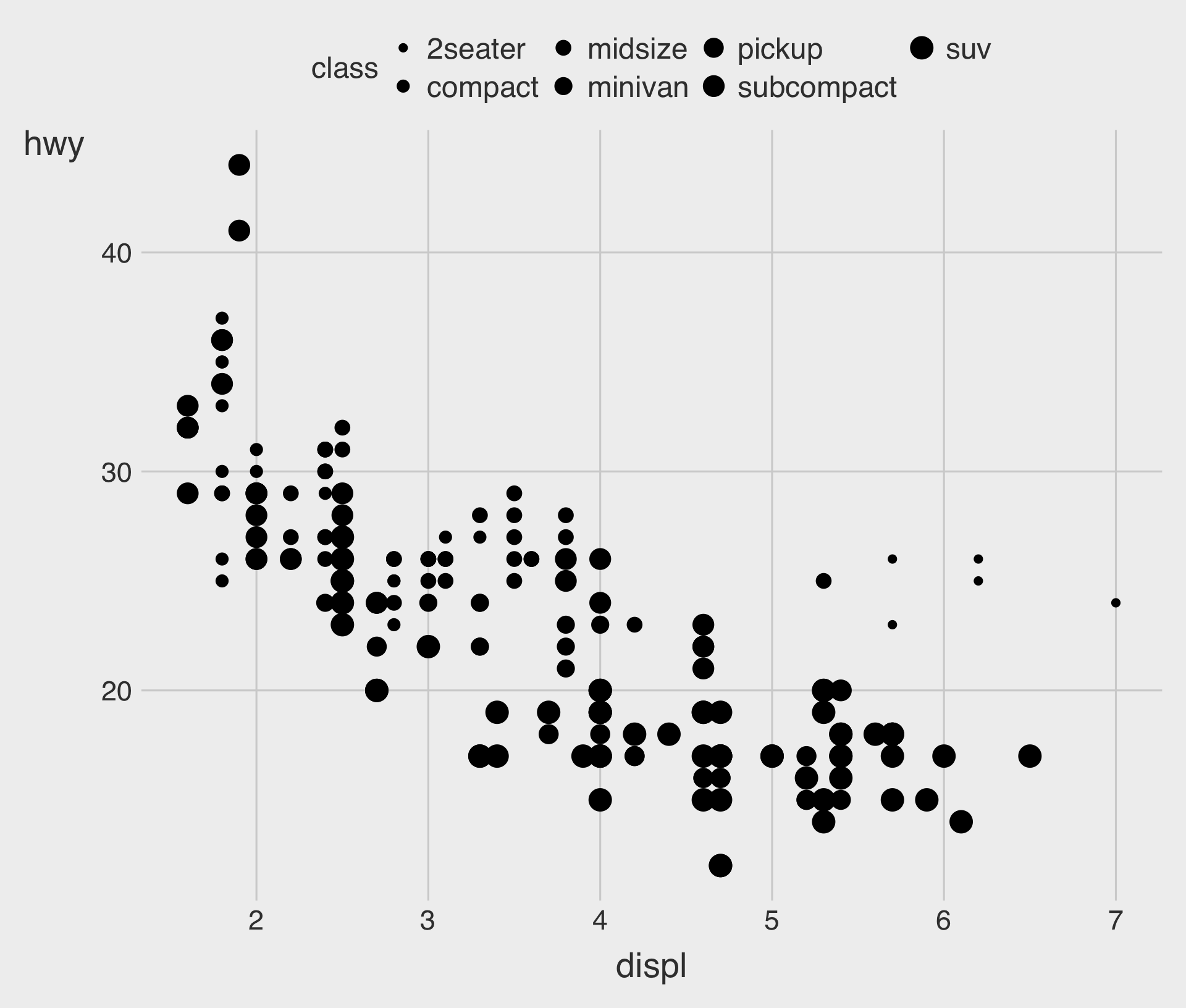
Adding a size to the Plot
Specifying a color to the Plot, Manually
Specifying a color to the Plot, Manually
Specifying a fill to the Plot, Manually
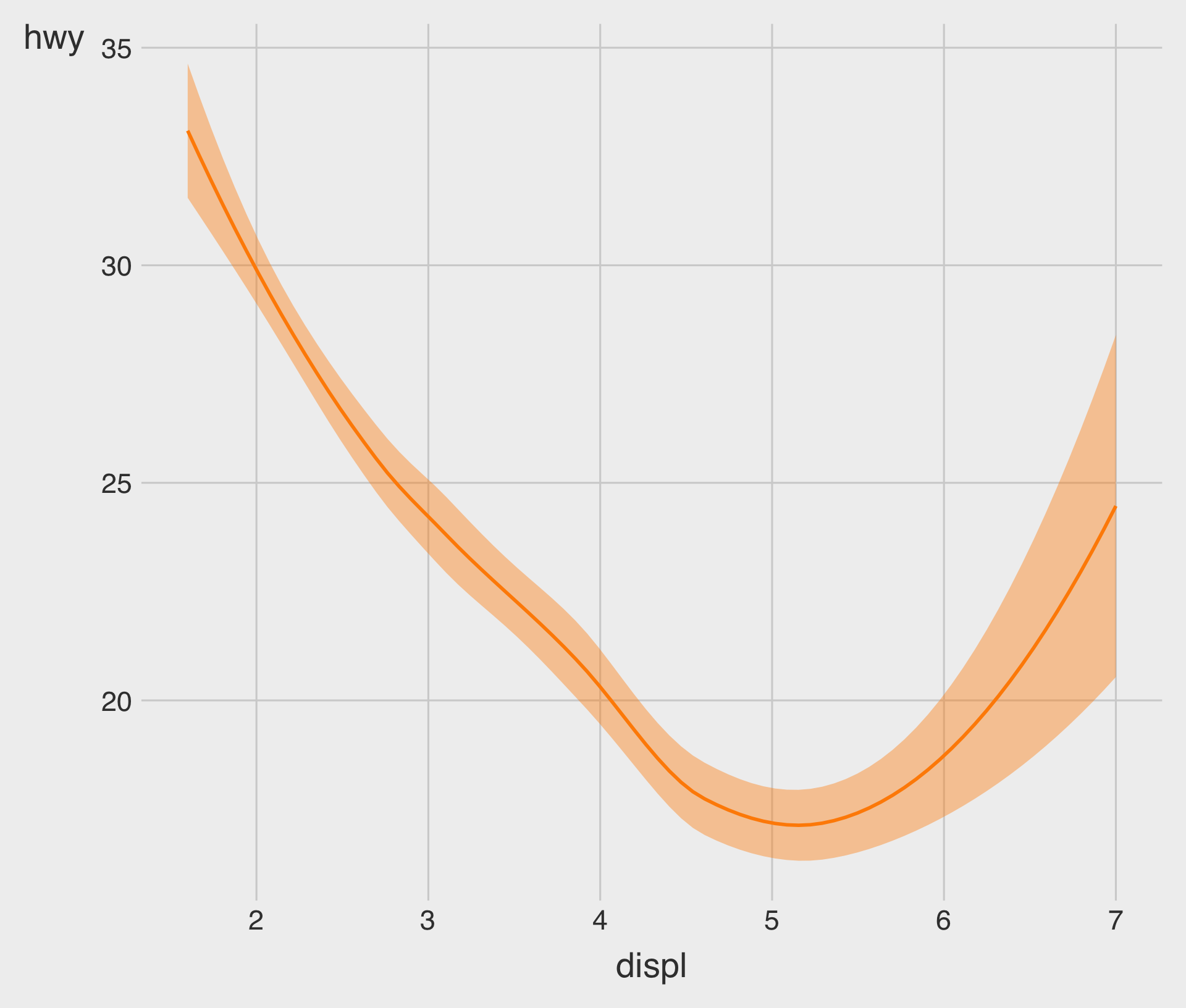
- In general, each
geom_*()has a different set of aesthetic parameters.- E.g.,
fillis available forgeom_smooth(), but notgeom_point()in general (cf., Aesthetics Finder).
- E.g.,
Specifying a size to the Plot, Manually
Specifying a shape to the Plot, Manually

Specifying a shape to the Plot, Manually
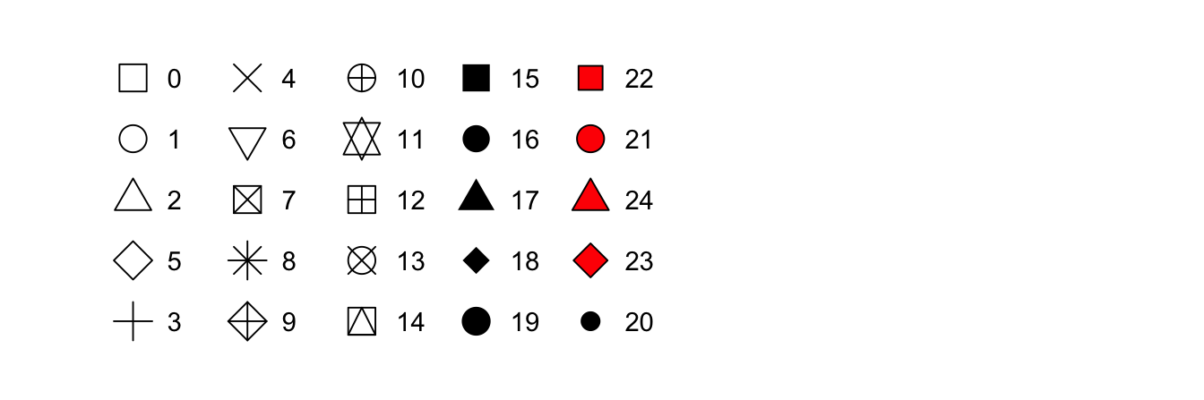
- In ggplot2, point shapes are specified using numbers, as shown above.
- R provides 26 built-in point shapes, identified by integers
0–25.
- R provides 26 built-in point shapes, identified by integers
Specifying an alpha to the Plot, Manually
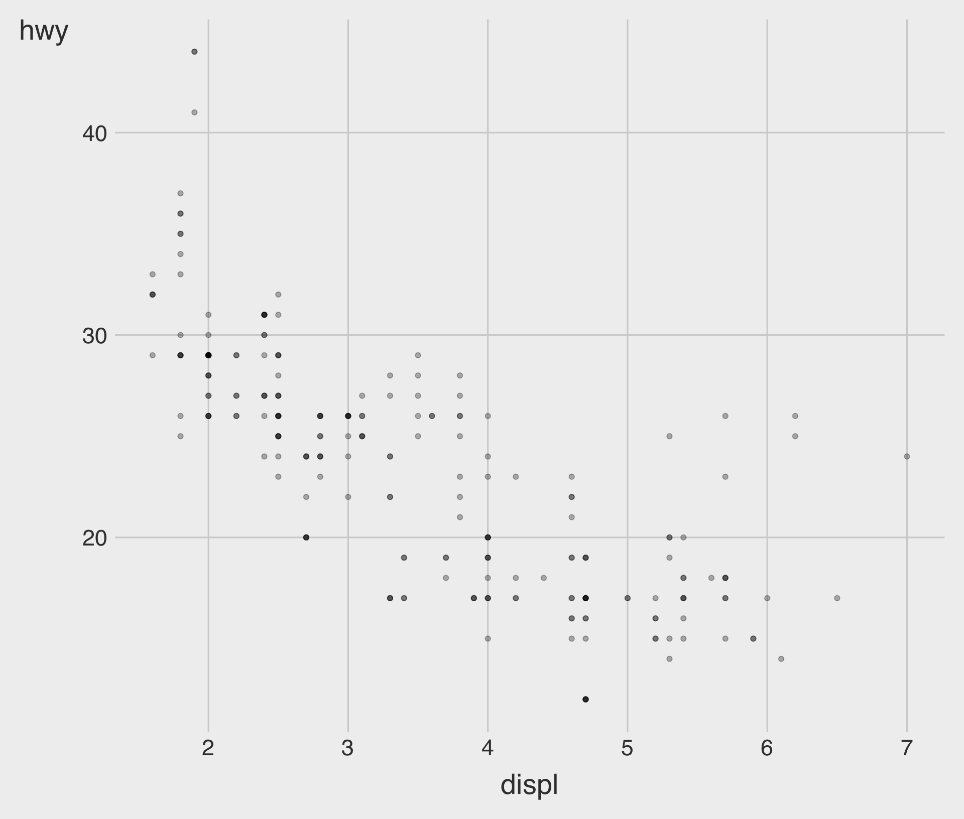
- We’ve done this to address the issue of overplotting in the scatterplot.
Multiple data.frames and aes() in ggplot
Clutter is Your Enemy!
- Which one do you prefer?
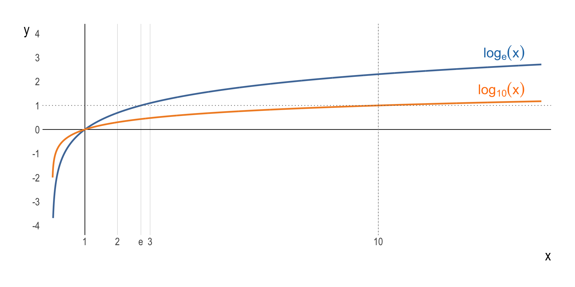
A Little Bit of Math for Logarithm
- The logarithm function, \(y = \log_{b}\,(\,x\,)\), looks like ….
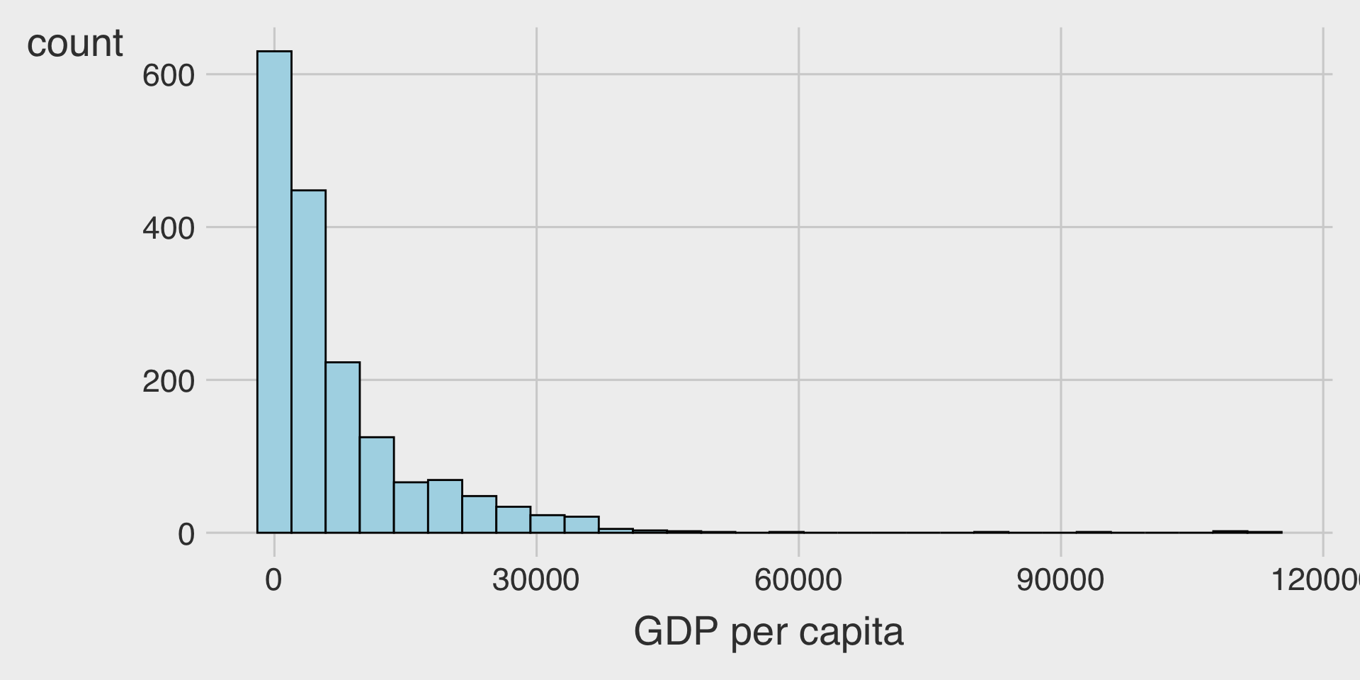
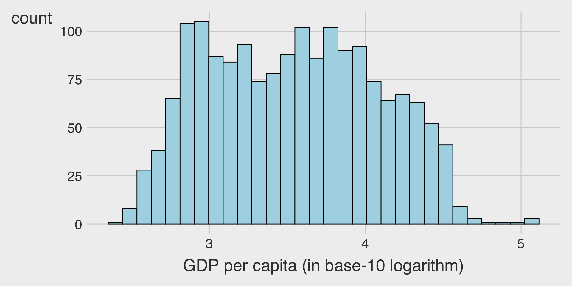
The Use of Logarithms: Handling Skewed Data
- Consider a logarithmic scale when a variable is heavily skewed.
- It helps visualize both small and large values effectively.
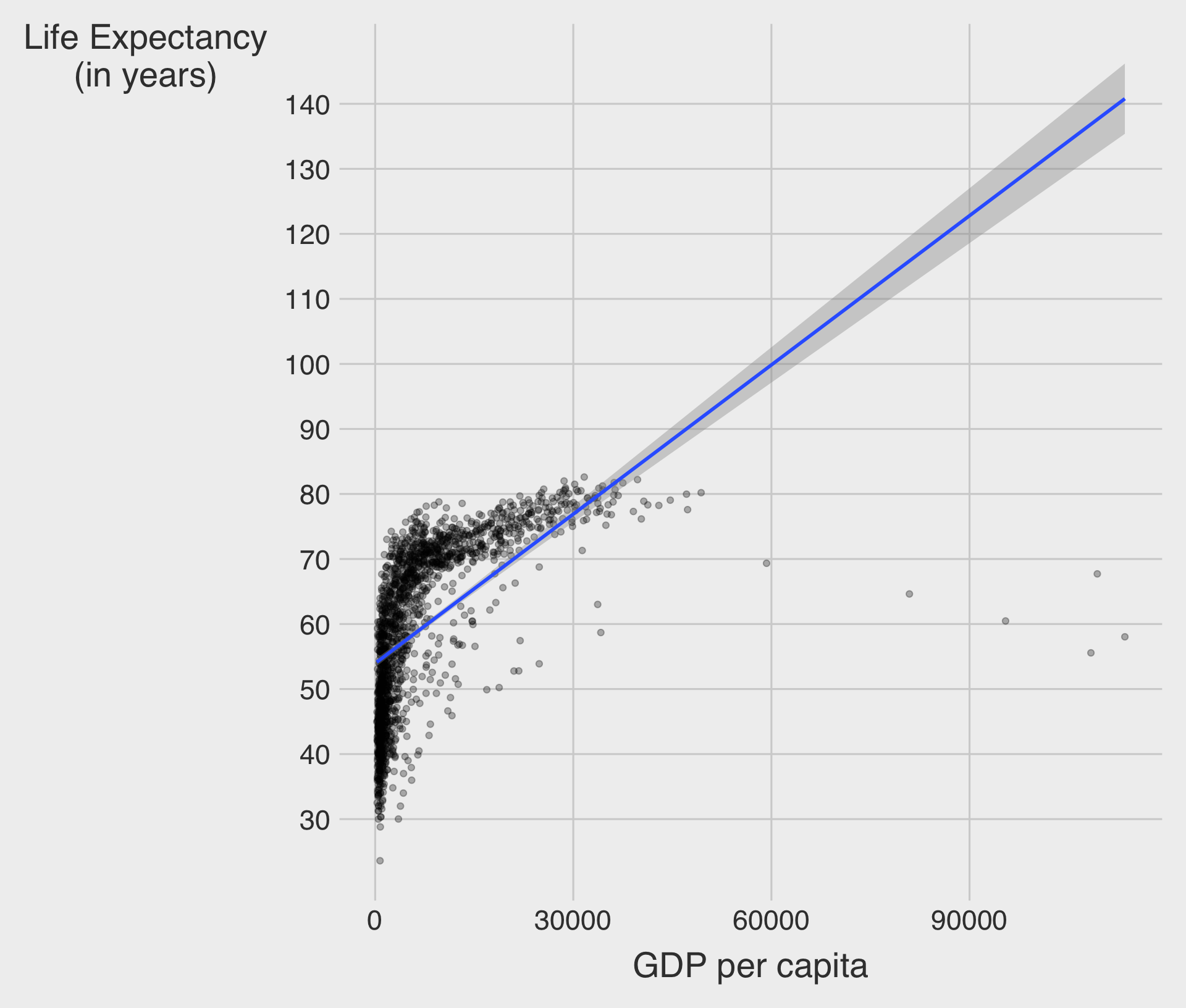
Without Log Transformation
With Log Transformation
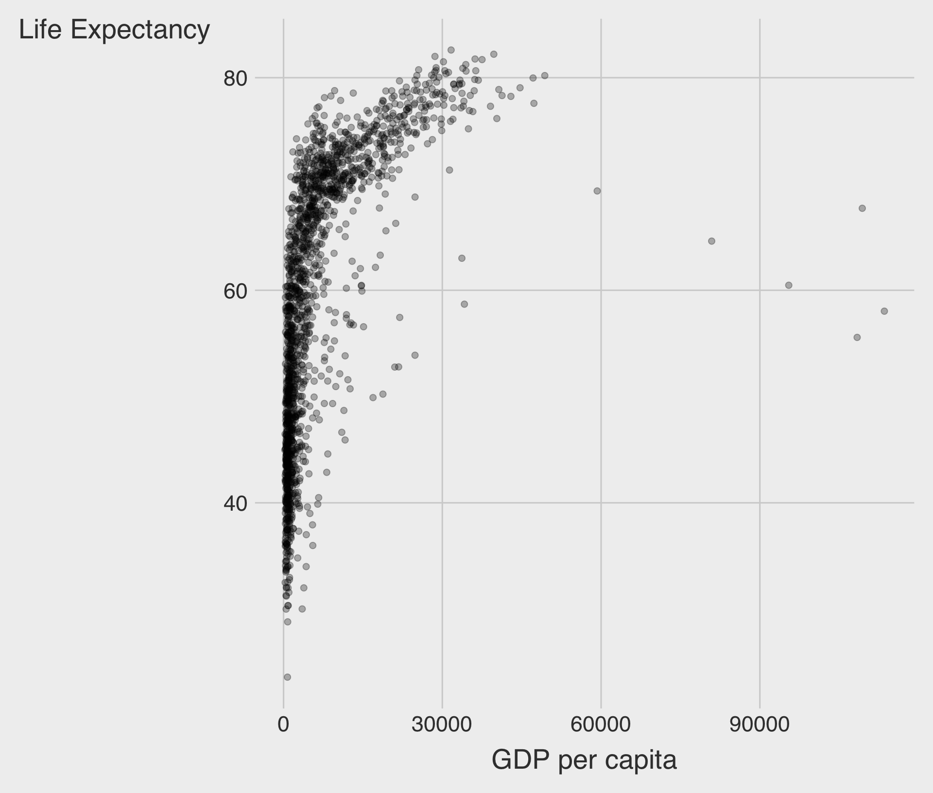
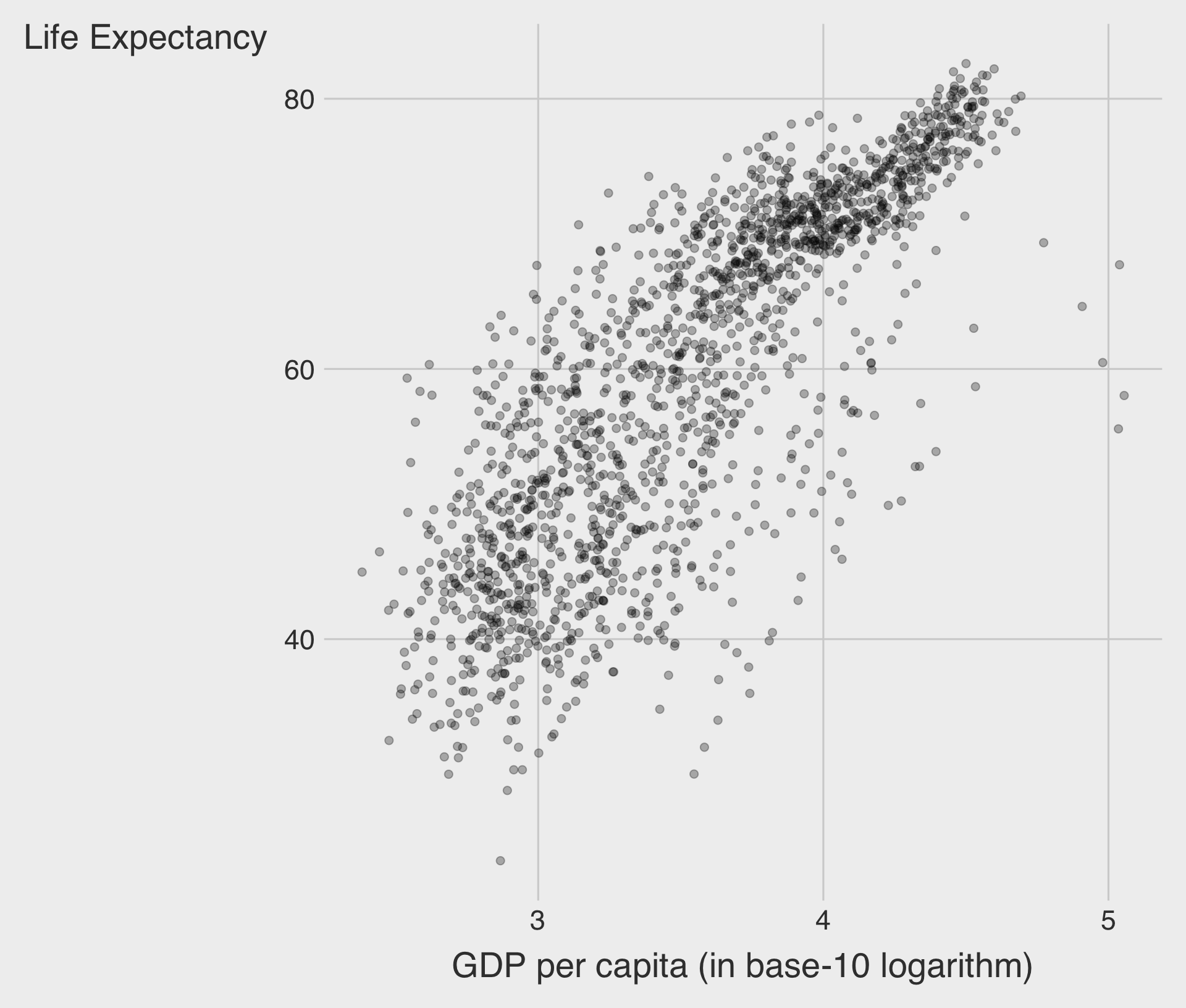
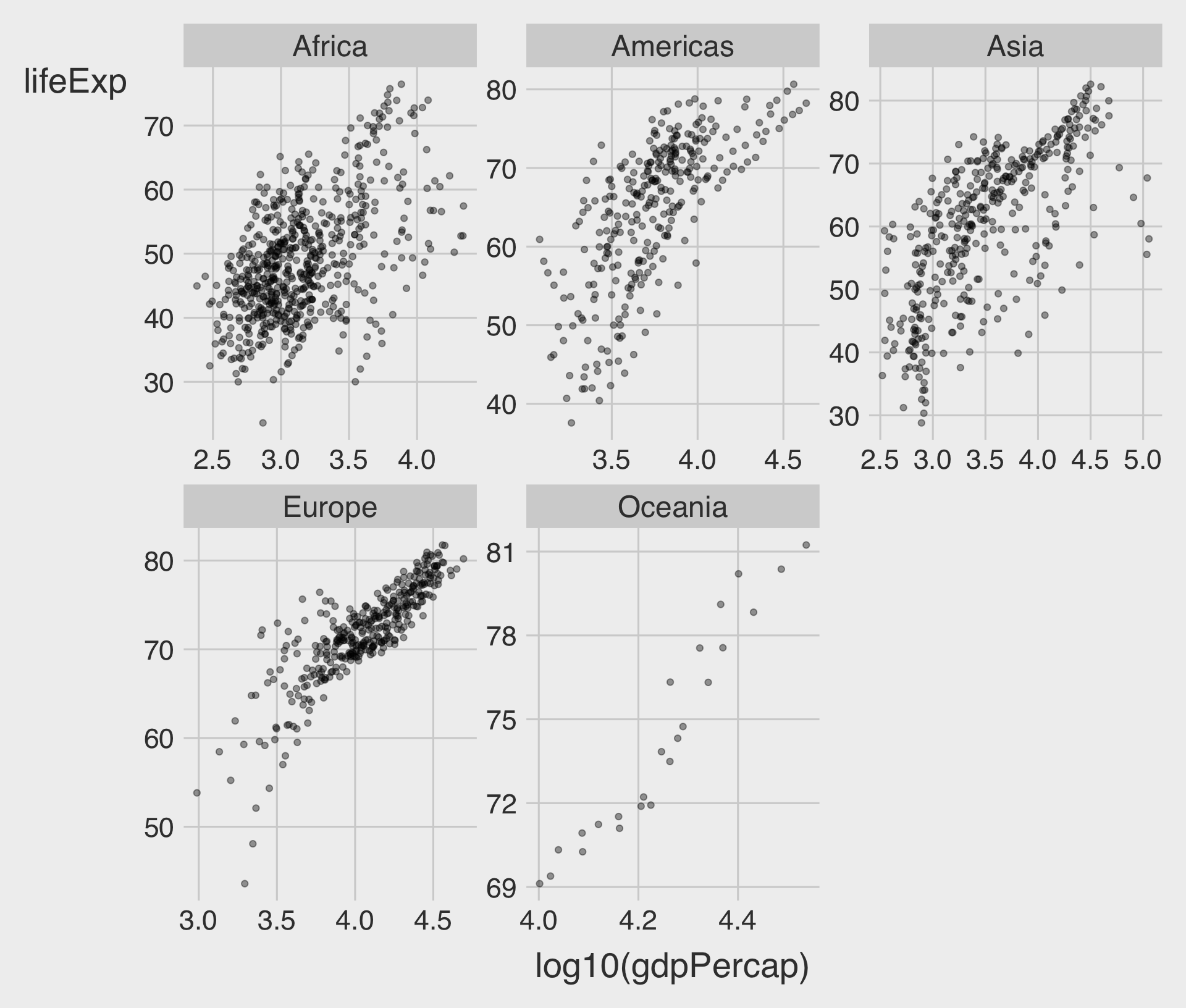
🌍 Example: GDP per Capita vs. Life Expectancy
Linear Scale
Log Scale
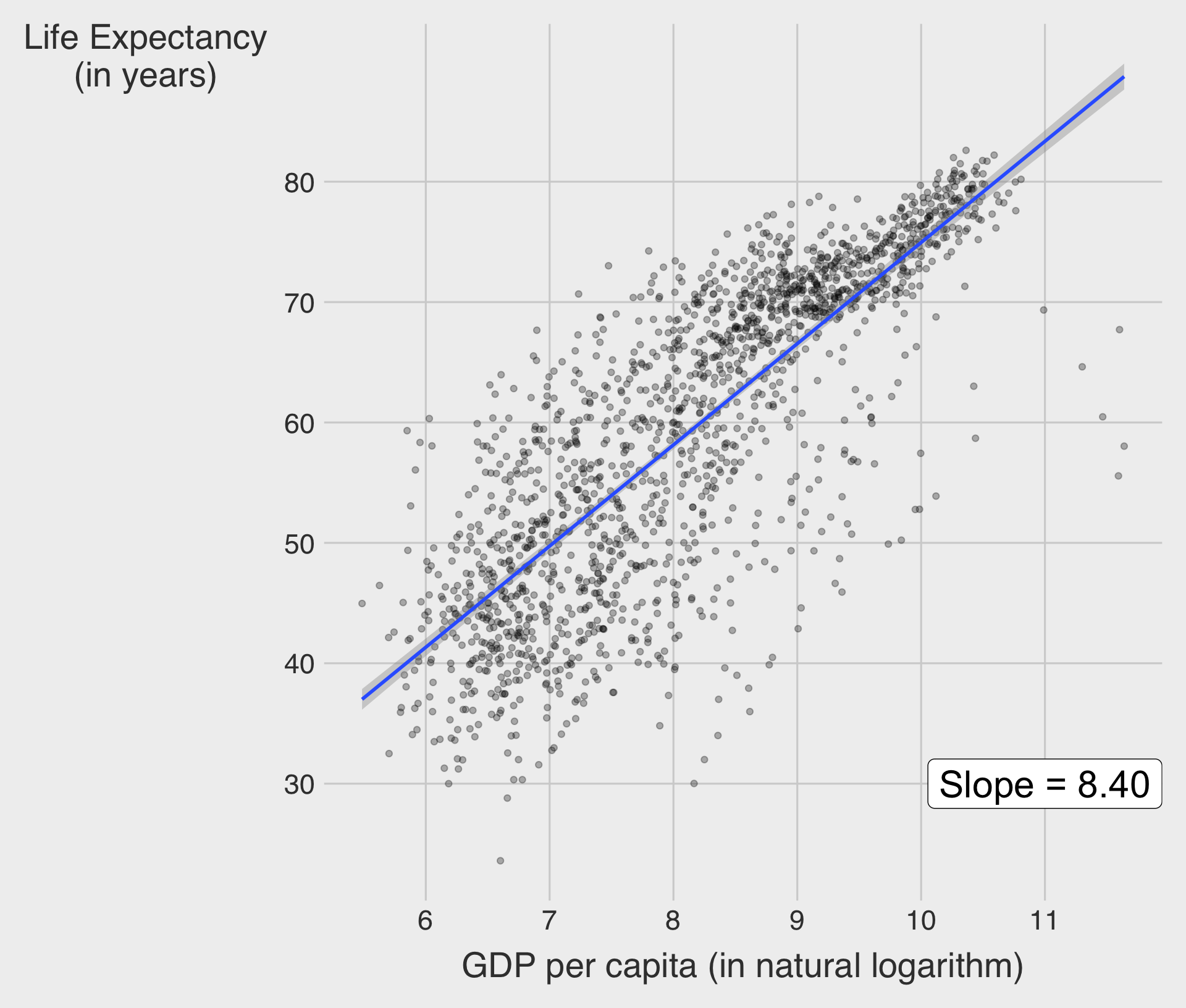
- ✅ Slope = 8.4 : \(\;\) A 1-unit increase of log(GDP per capita) is associated with an increase in life expectancy of about 8.4 years.
- A 1% increase in GDP per capita is associated with an increase in life expectancy of about 0.084 years (≈ 30.7 days).
Try it out → Classwork 2: Relationship Plots.
Facets
- Adding too many aesthetics (e.g.,
color,shape,size) can sometimes make a plot cluttered and hard to interpret.
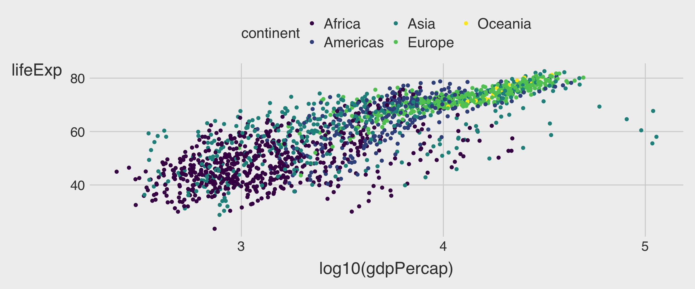
- To incorporate an additional variable, especially a categorical one, we can use facets — separate subplots that each show a subset of the data.
- Faceting helps reveal patterns within groups while keeping each plot clean and focused.
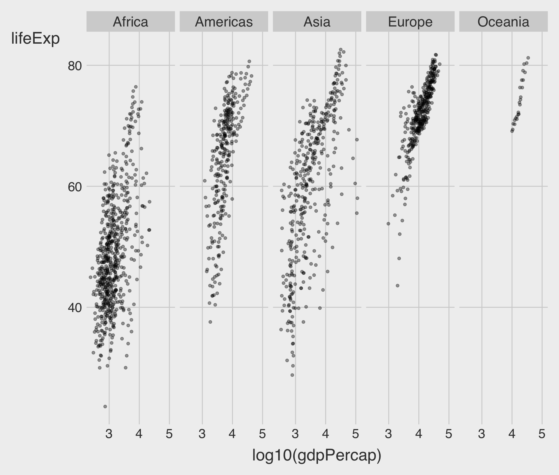
facet_wrap(~ VAR)
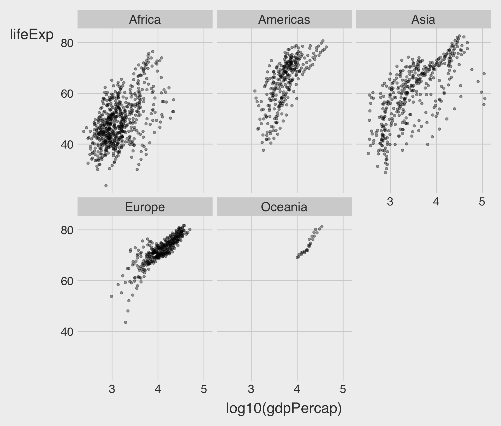
- To facet our plot by a single variable, we can use
facet_wrap().
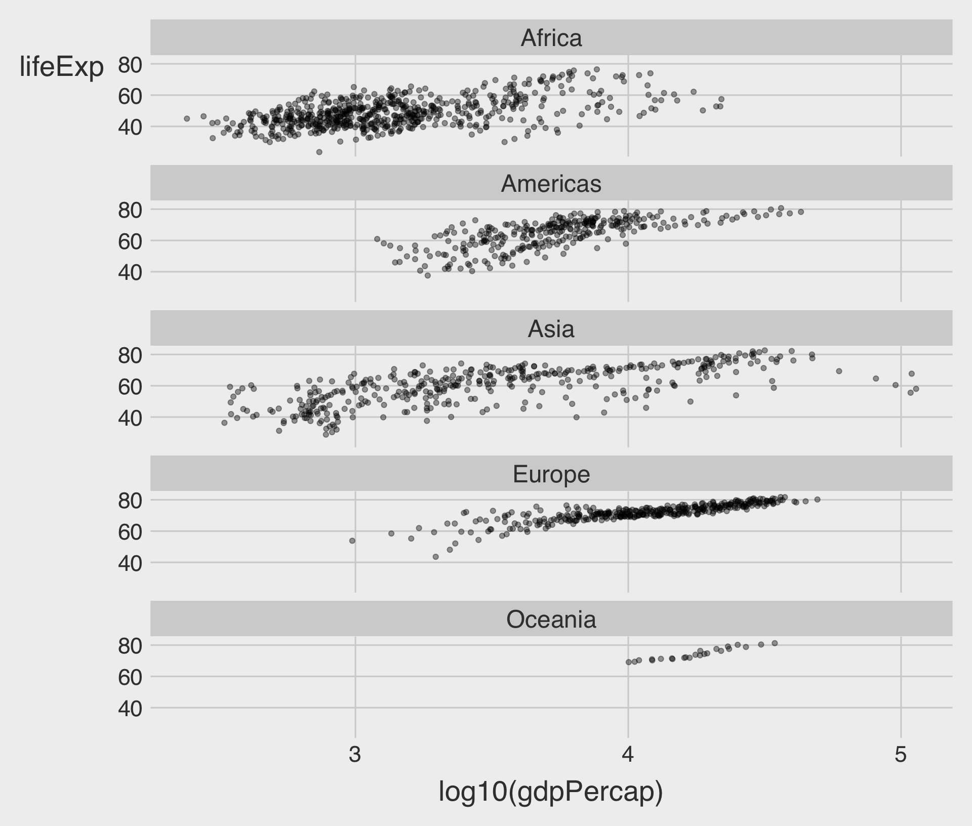
facet_wrap(~ VAR) with nrow
nrowdetermines the number of rows to use when laying out the facets.
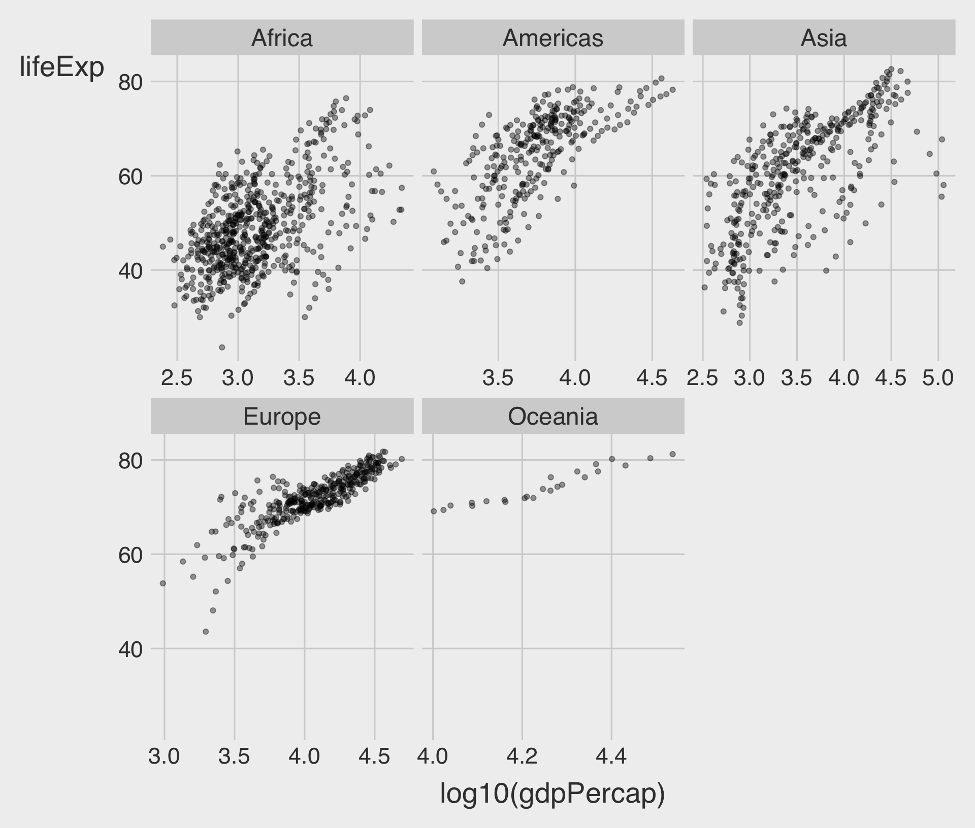
facet_wrap(~ VAR) with ncol
ncoldetermines the number of columns to use when laying out the facets.
facet_wrap(~ VAR) with scales = "free_x"
scales = "free_x"allow for different scales of x-axis
facet_wrap(~ VAR) with scales = "free_y"
scales = "free_y"allow for different scales of y-axis
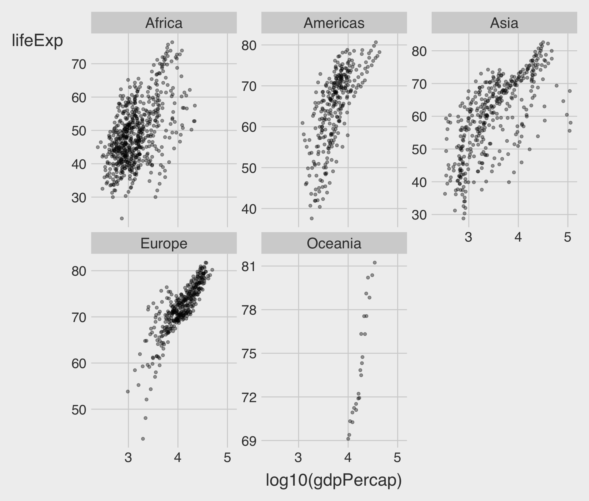
facet_wrap(~ VAR) with scales = "free"
scales = "free"allow for different scales of both x-axis and y-axis- Try it out → Classwork 3: Color vs. Facet.
facet_grid(ROW ~ COL)
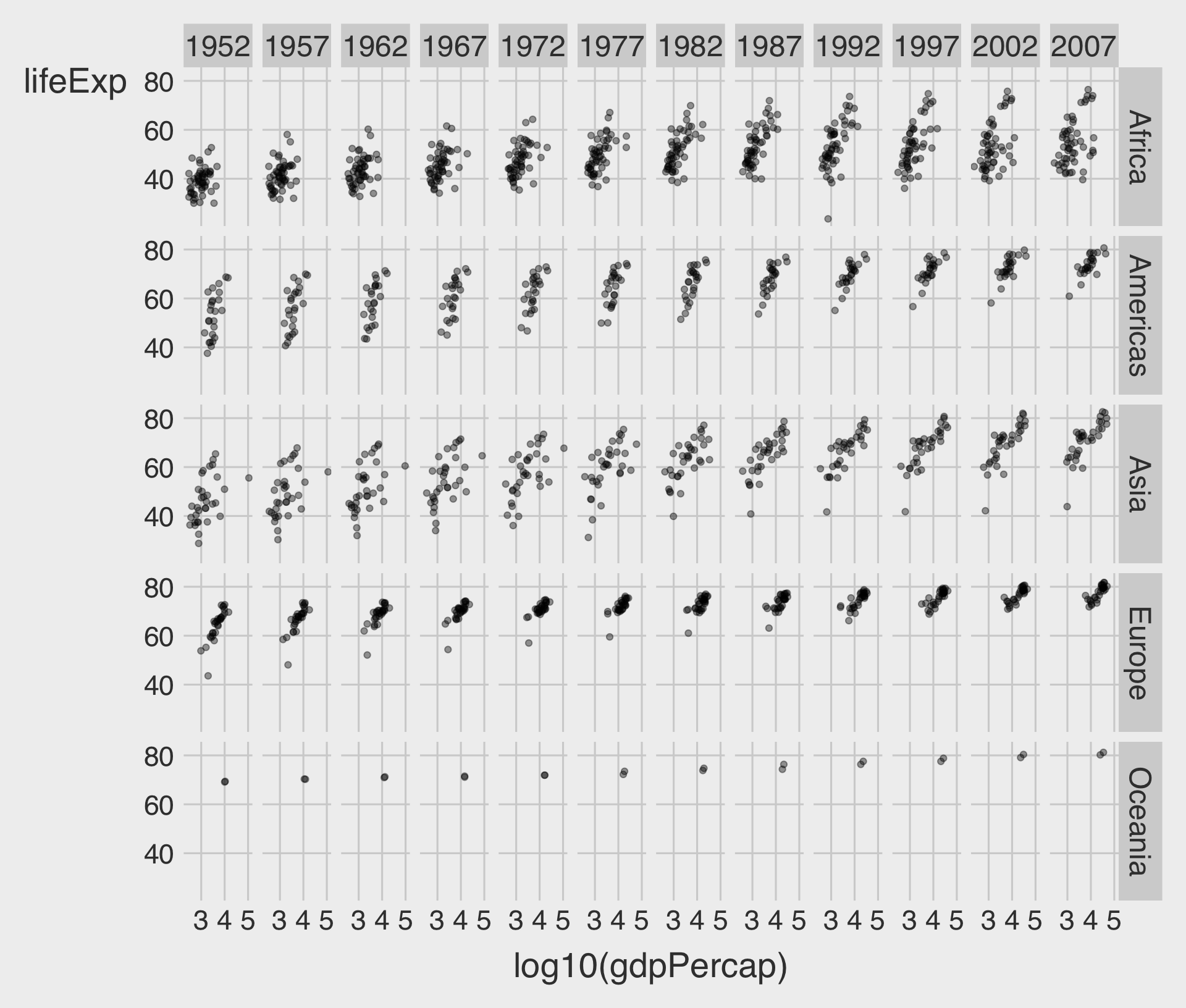
- To facet by two variables (rows and columns), use
facet_grid(ROW ~ COL). - Each row is a level of continent, and each column is a level of year.
nrow,ncol, andscalesoptions also work withfacet_grid()
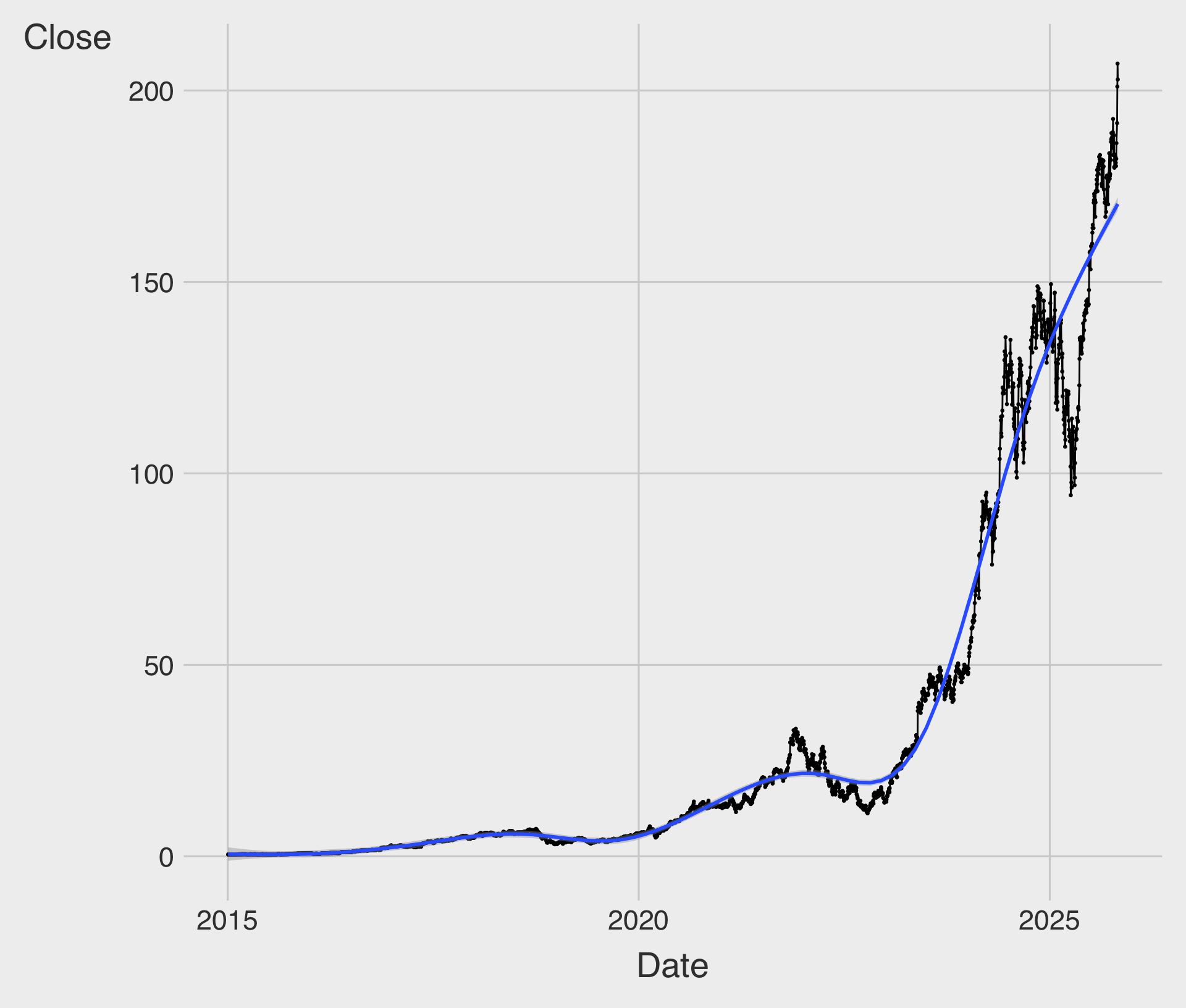
Scatterplot for Time Trend?
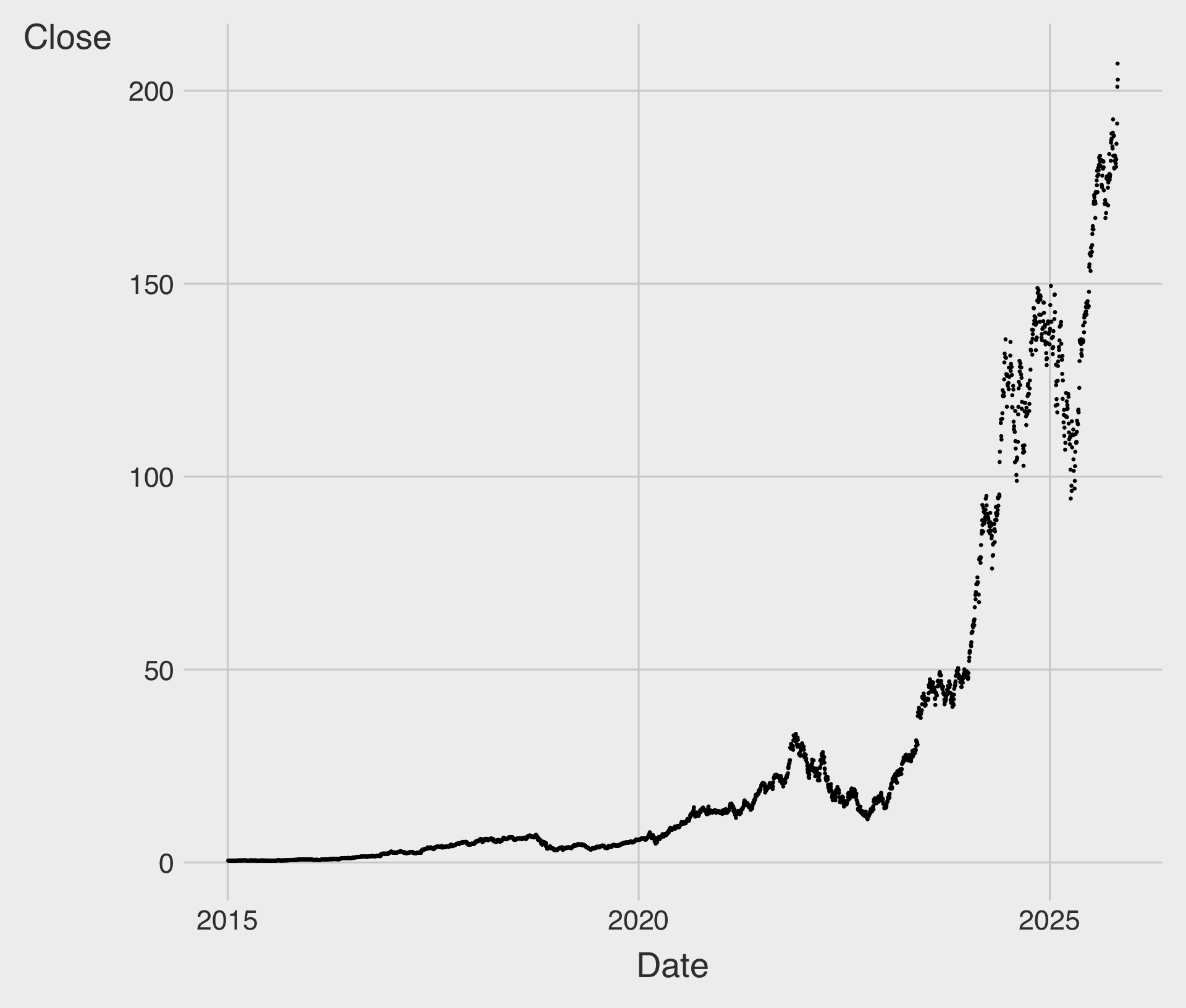
Line Chart with geom_line()
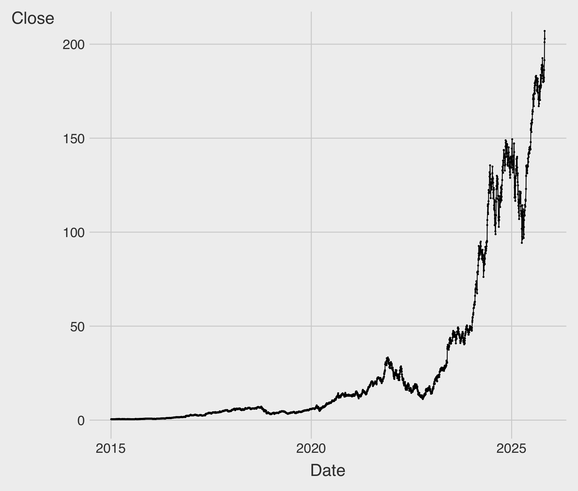
geom_line()draws a line by connecting data points in order of the variable on thex-axis.
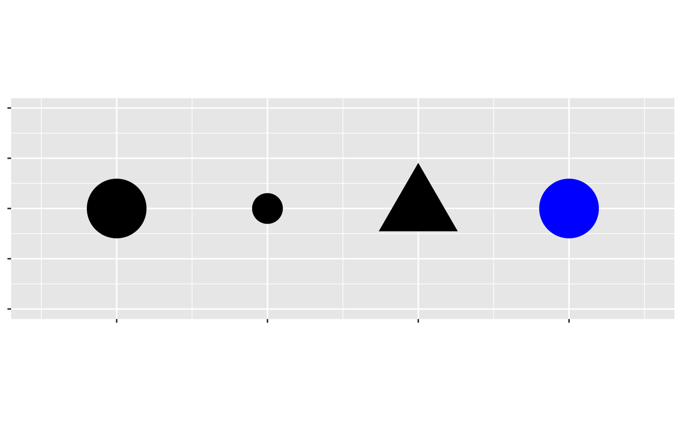
The Connection Principle
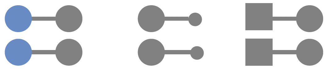
- We tend to think of objects that are physically connected as part of a group.
- Look at this figure.
- Your eyes probably pair the shapes connected by lines rather than similar color, size, or shape!
- We frequently leverage the connection principle is in line charts, to help our eyes see order in the data.
Line Chart with geom_line() and geom_smooth()
geom_smooth()helps reveal underlying long-term trends by smoothing out variability in the observations.
Time Trend of Tech Stock Price
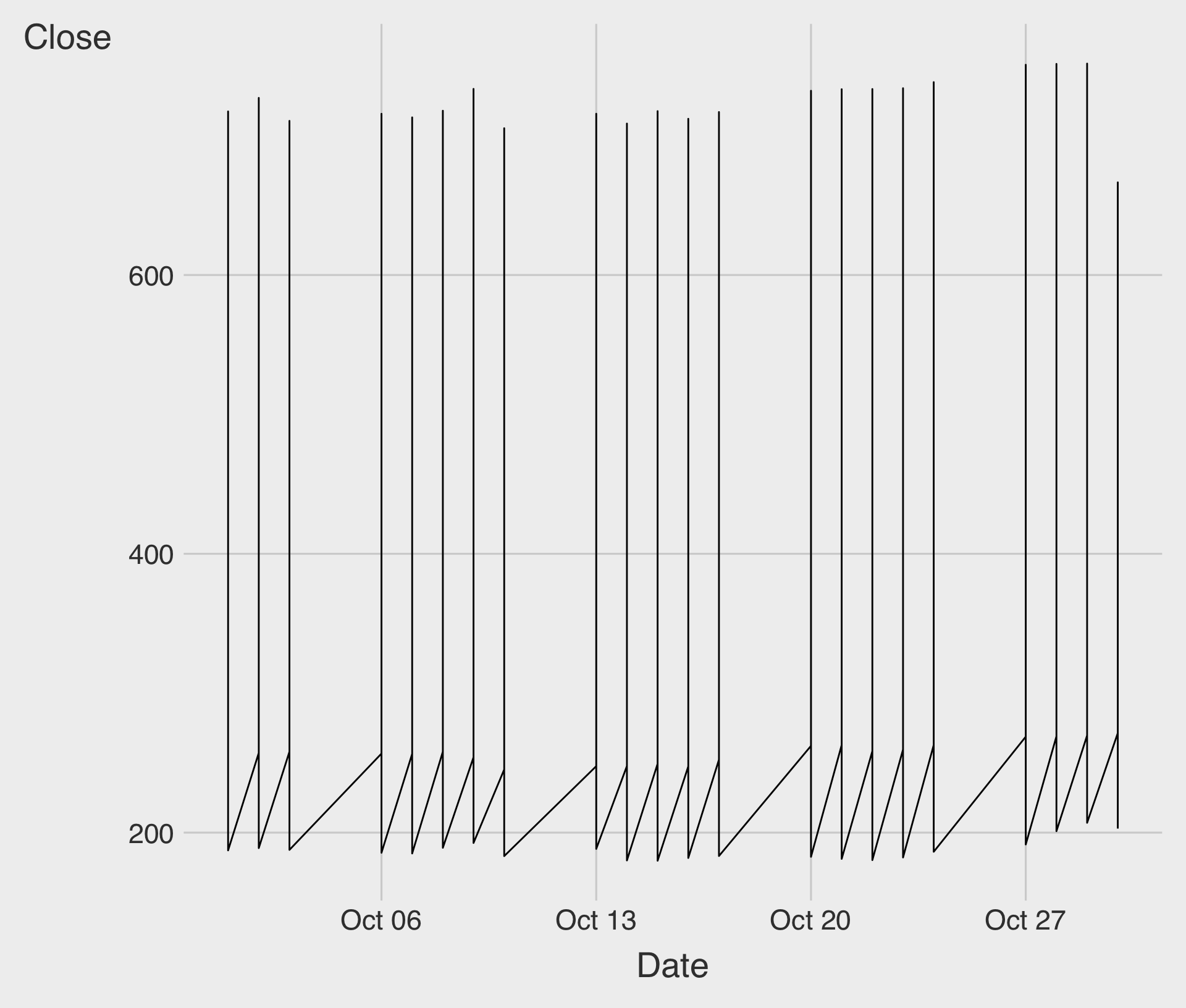
- Something has gone wrong. What happened?
Time Trend of Tech Stock Price
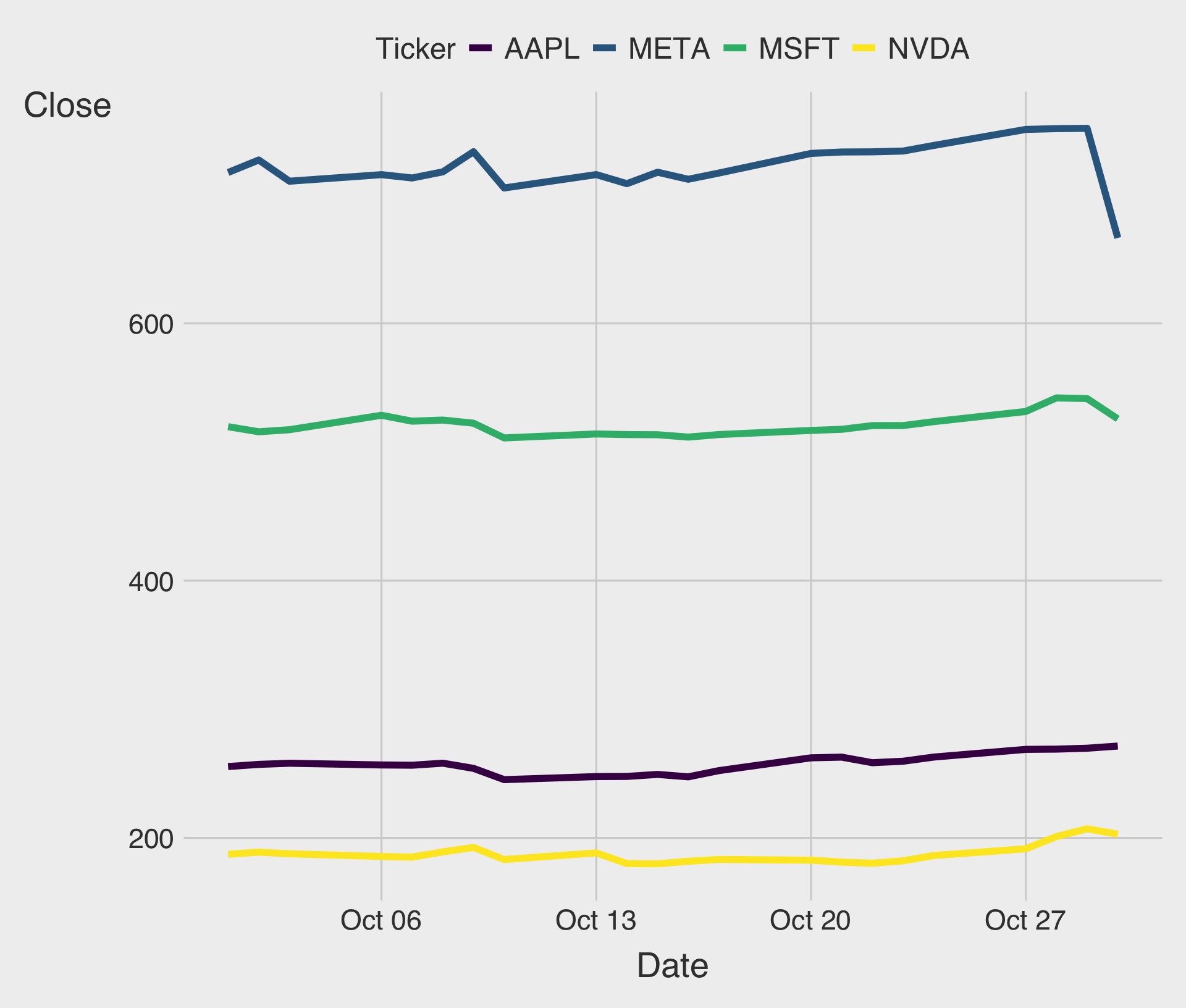
We can use the
group,color, orlinetypeaesthetic to tell ggplot about the firm-level grouping structure in the dataset.Try it out → Classwork 4: Time Trend Plots.
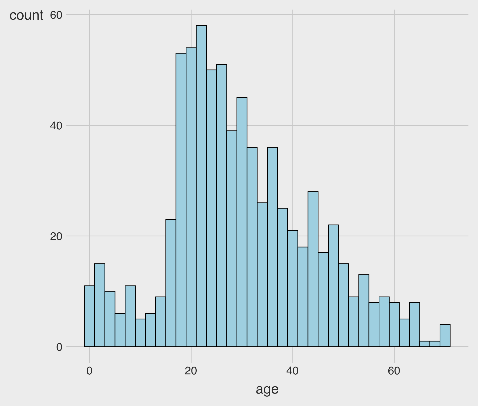
Histograms
Histograms are used to visualize the distribution of a numeric variable.
Histograms divide data into bins and count the number of observations in each bin.
Histograms with geom_histogram()
geom_histogram()creates a histogram.- We map the
xaesthetic to a variable.
- We map the
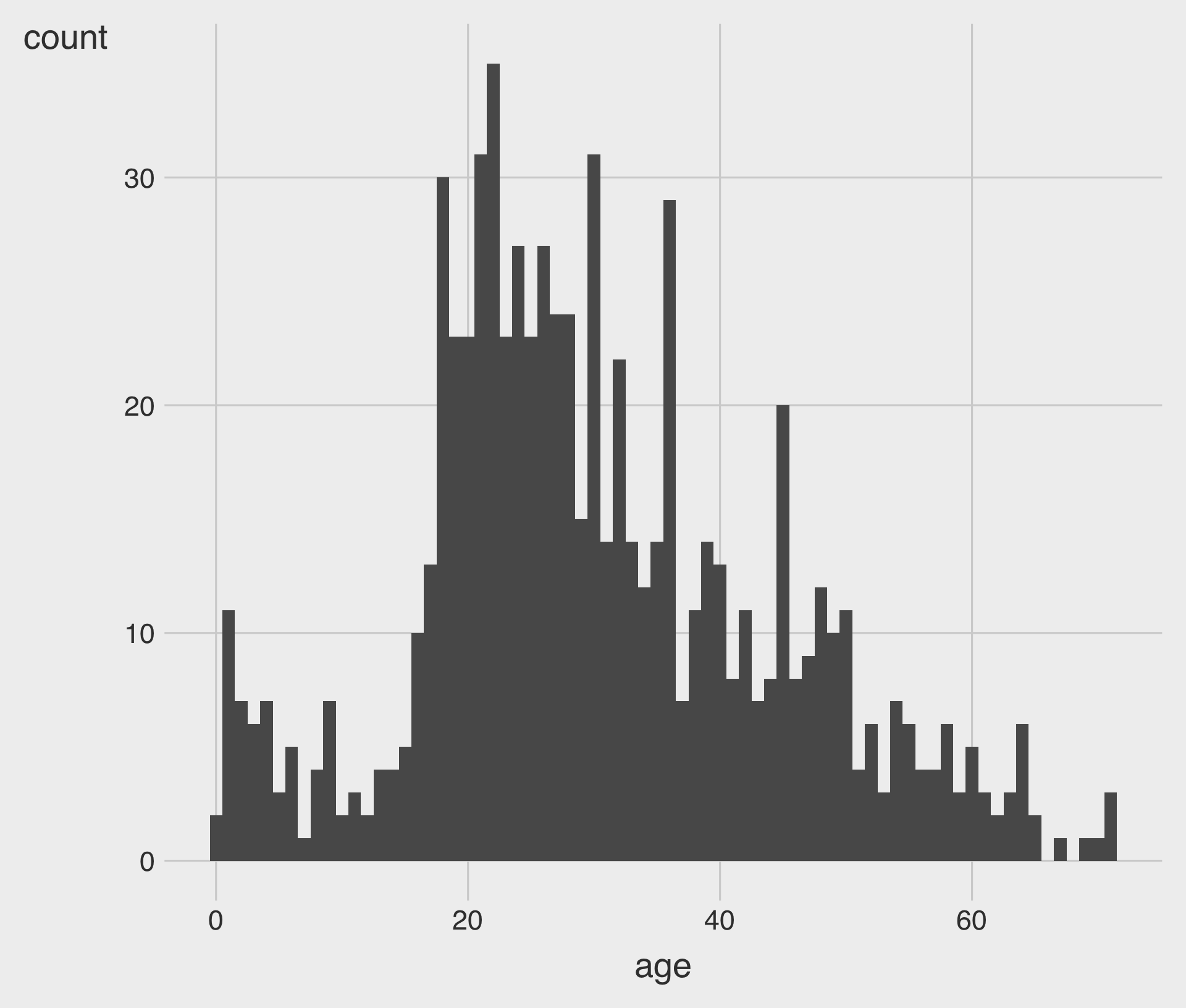
geom_histogram() with bins
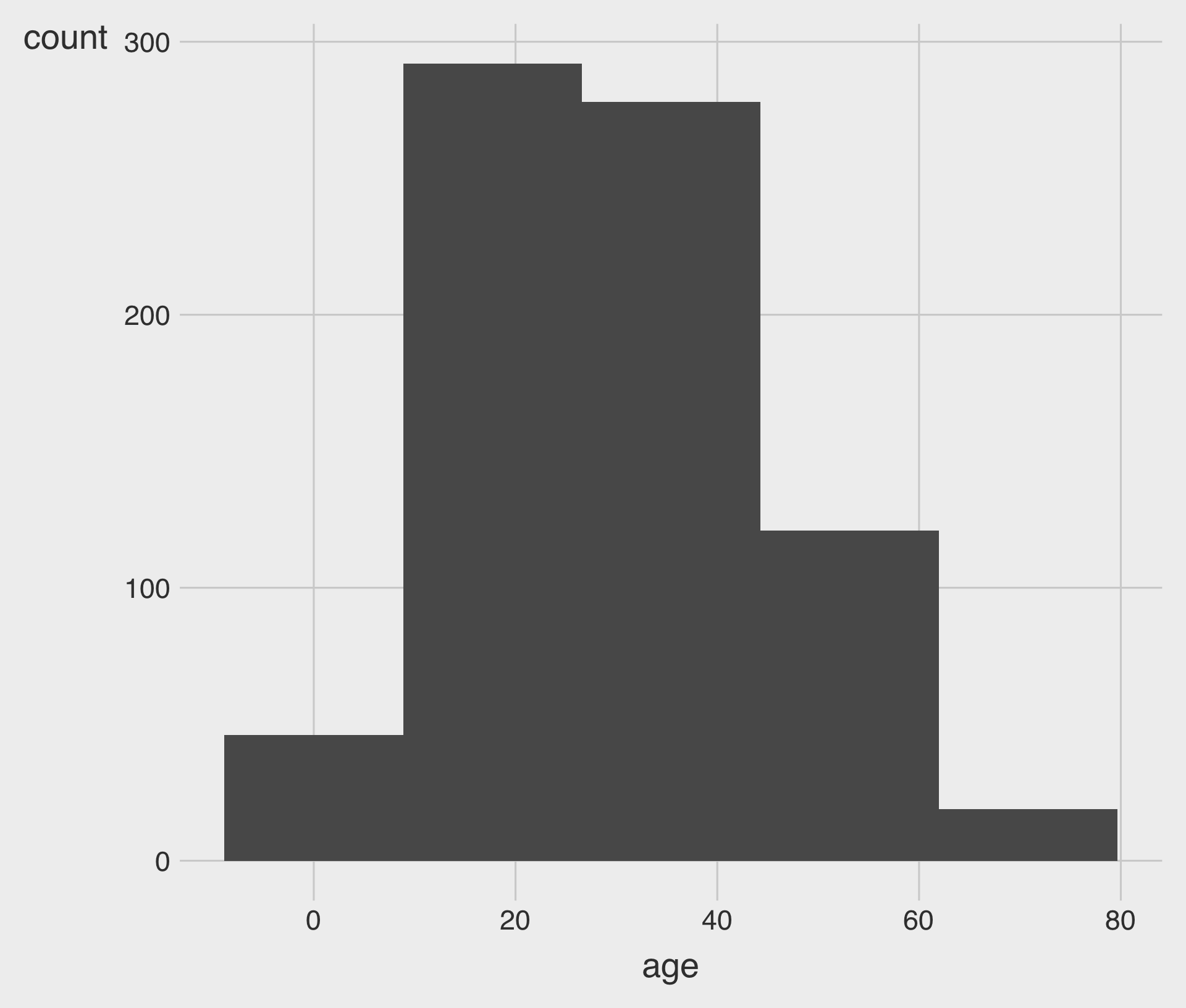
bins: Specifies the number of bins- Be careful: the number of bins can greatly influence the shape of a histogram.
geom_histogram() with binwidth
binwidth: Specifies the width of each bin- We choose either the
binsoption or thebinwidthoption.
Customizing the color and fill Aesthetics
fill: Fills the bars with a specific color.color: Adds an outline of a specific color to the bars.
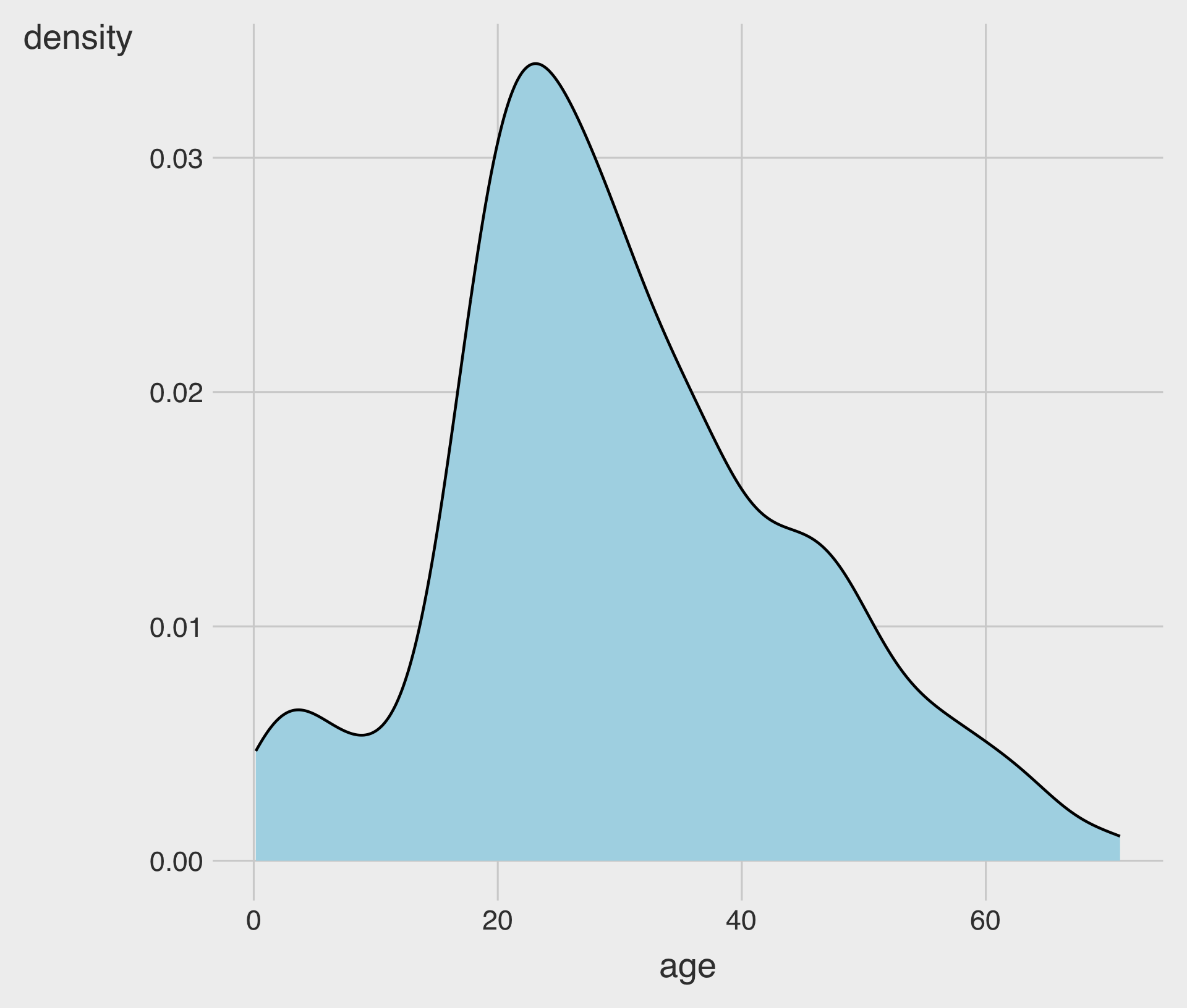
Kernel Density with geom_density()
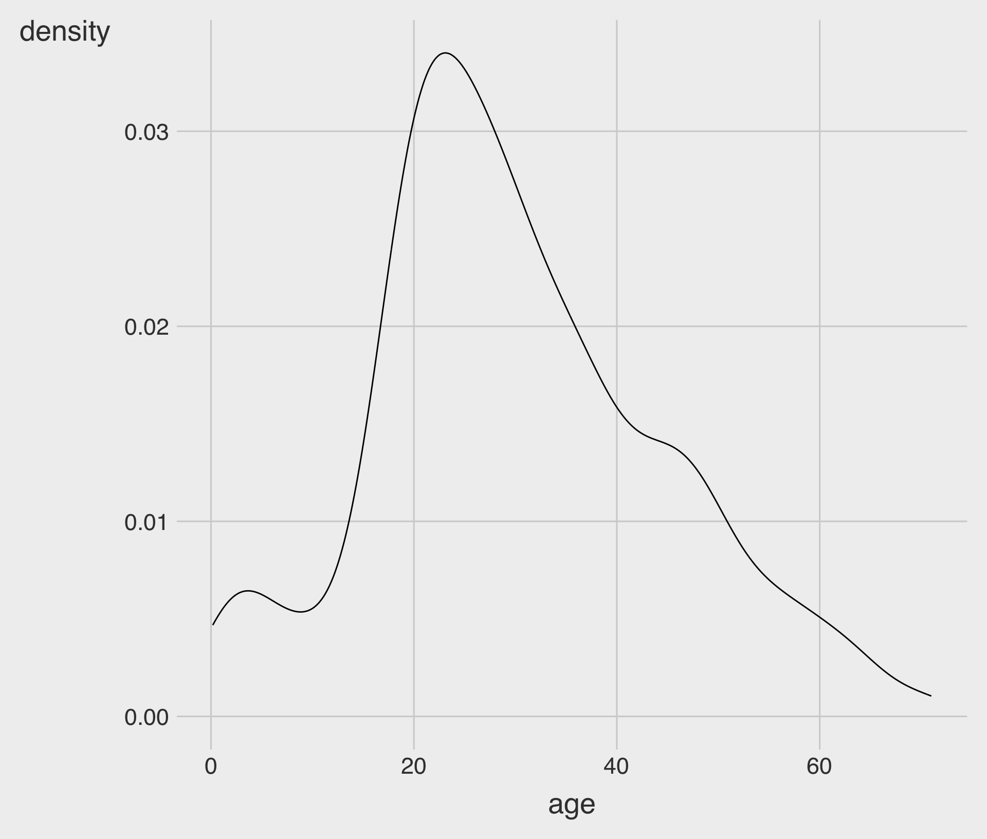
geom_density()creates a kernel density curve.- We map the
xaesthetic to a numeric variable.
- We map the
Customizing the color and fill Aesthetics
fill: fills the area under the curvecolor: controls the outline color of the curvelinewidthcontrols outline thickness
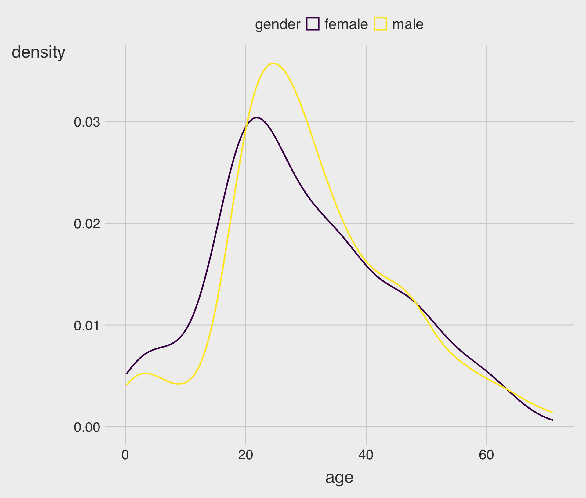
Mapping color (Outline) to a Group Variable
- Mapping
color = genderdraws multiple curves, one per group.
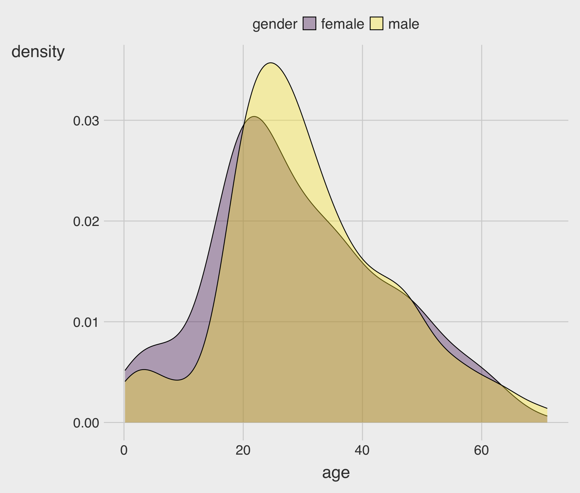
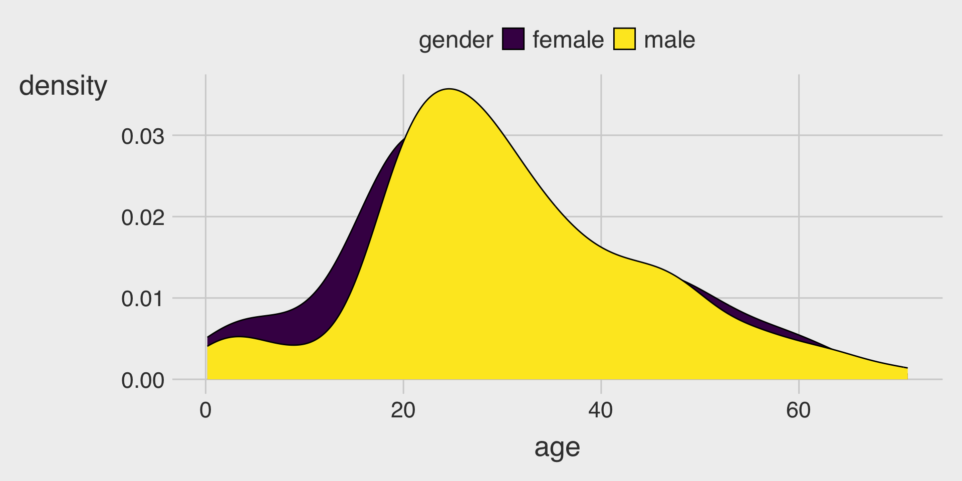
Mapping fill to a Group Variable (Overlapping Distributions)
- When multiple filled curves overlap, use transparency (
alpha) so you can see both.
Mapping color to a Group Variable with geom_freqpoly()
- A frequency polygon is a line-based version of a histogram that connects the heights of binned counts across the x-axis.
geom_freqpoly()does not supportfillaesthetic.
position = "identity" (Best for Comparison)

- Often the best choice when you want to compare shapes across groups.
- Use
alphato reduce clutter.
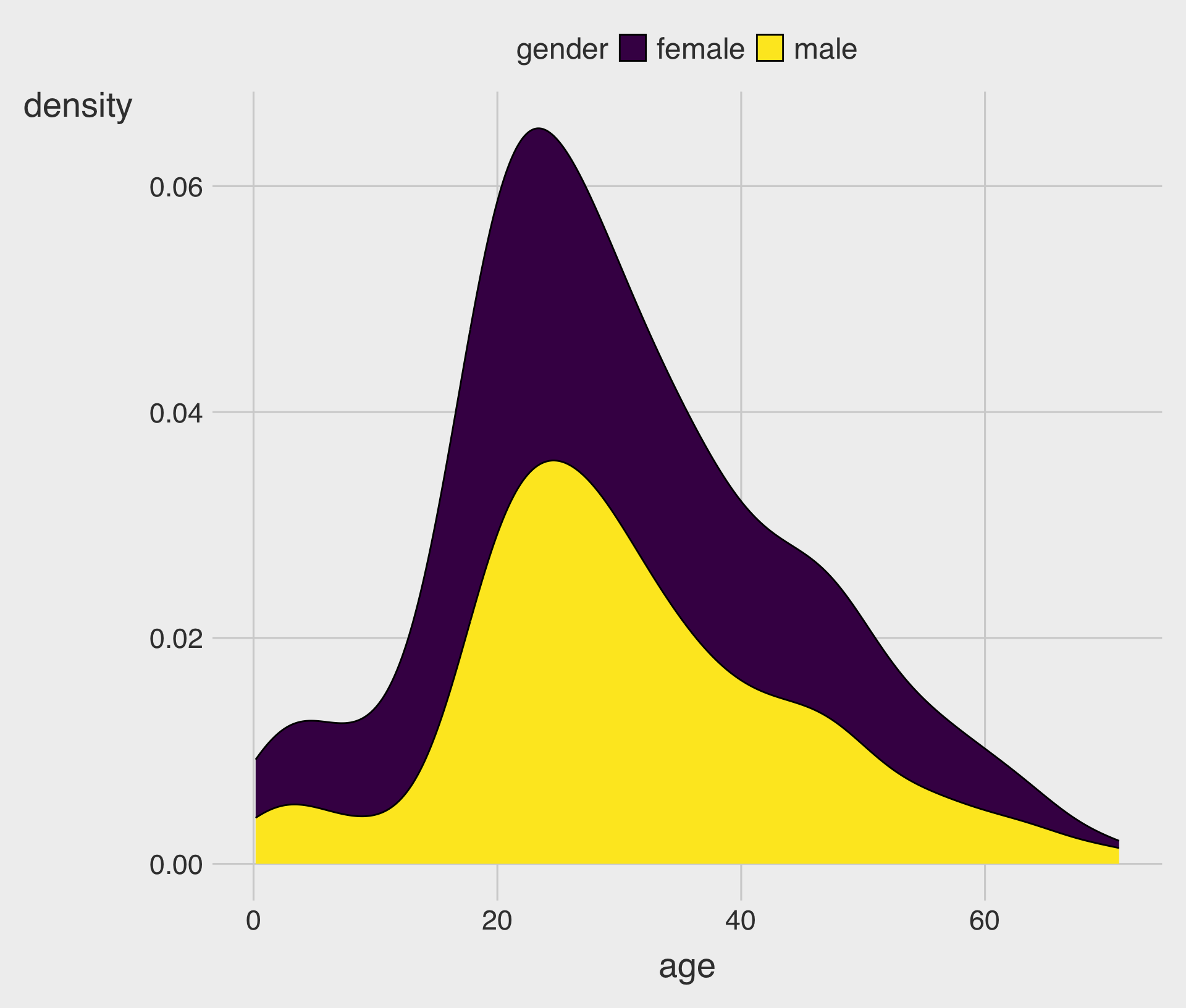
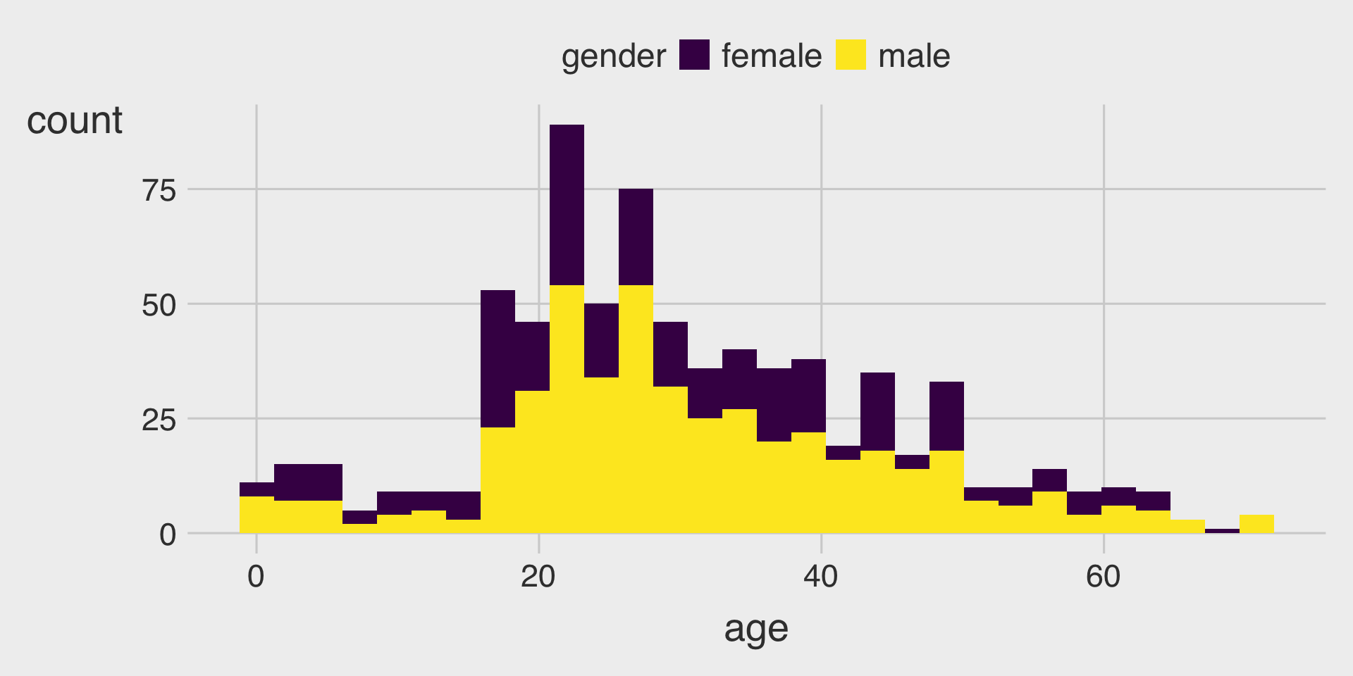
position = "stack" (Composition Emphasis)
- Highlights combined “mass” across groups.
- Not ideal for comparing group shapes directly (because the baseline shifts).
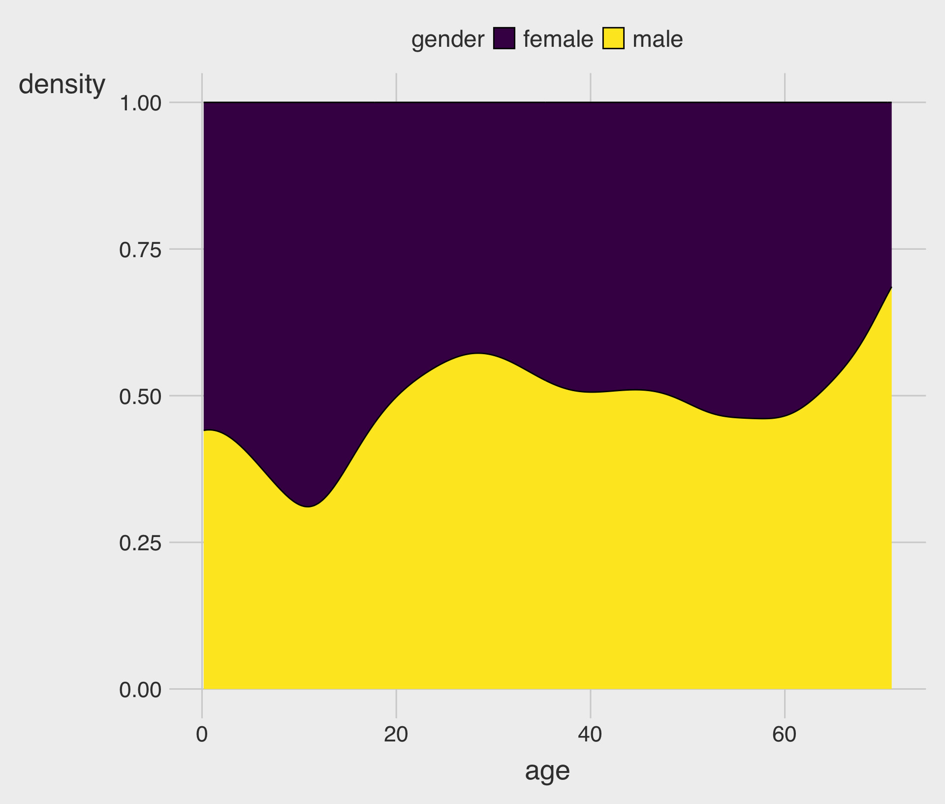
position = "fill" (Relative Composition Across x)
- At each
x-value, the stacked areas sum to 1 (100%). - Useful if you want “who dominates at each
xvalue?”
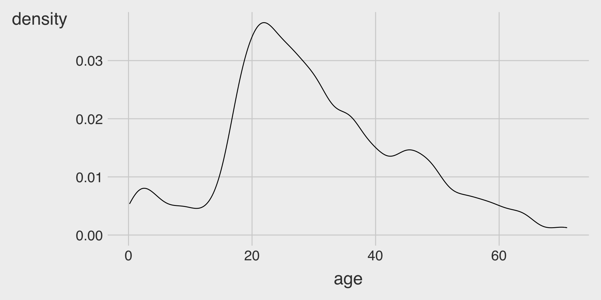
geom_density() with adjust

- Density smoothing depends on a bandwidth (how “wide” each kernel is).
- You can tune smoothing with
adjust(multiplies the default bandwidth)adjust < 1makes the curve less smoothadjust > 1makes the curve more smooth
Density vs Histogram with fill
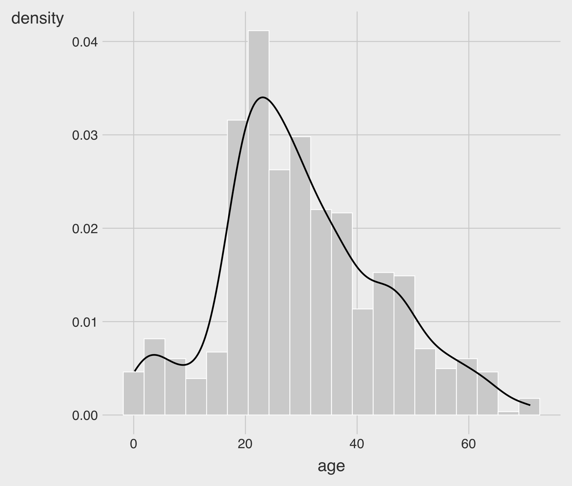
Density + Histogram Together
Sometimes it helps to overlay a density curve on top of a histogram.
aes(y = after_stat(density))rescales the histogram so the density curve matches the histogram scale.
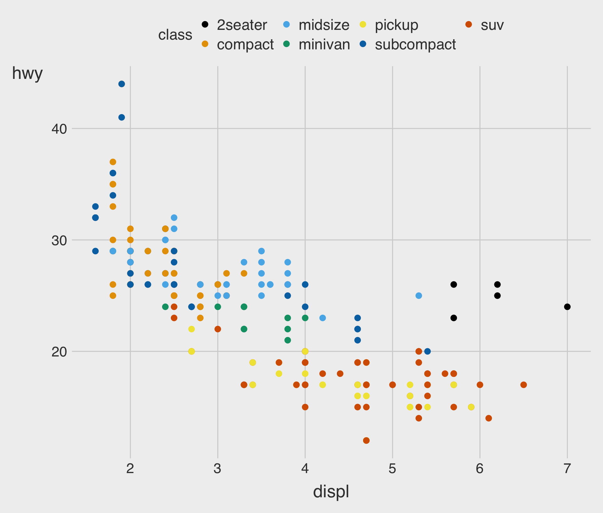
Design with Colorblind in Mind
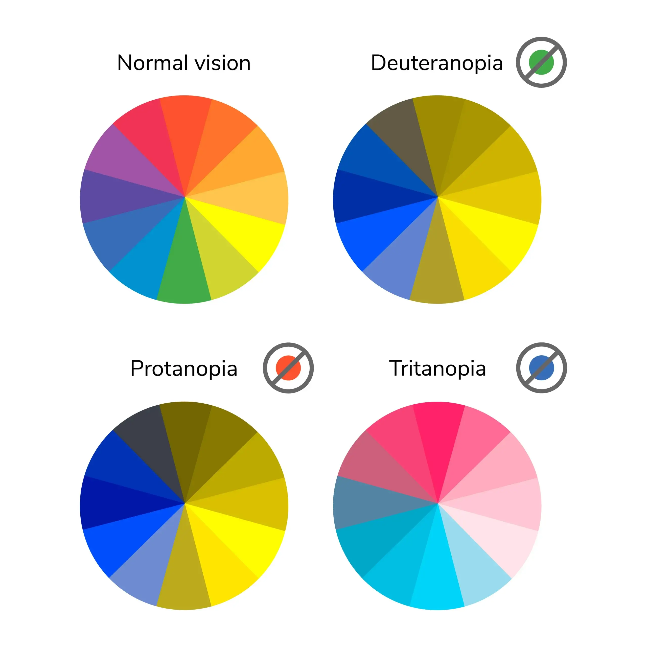
Types of Colorblindness
- About 8% of men and 0.5% of women experience some form of colorblindness.
- To make visualizations more accessible and colorblind-friendly, consider:
- Using colorblind-friendly palettes
- Adding
shapeto scatterplots orlinetypeto line charts - Including additional visual cues to highlight important information (e.g., annotations or labels)
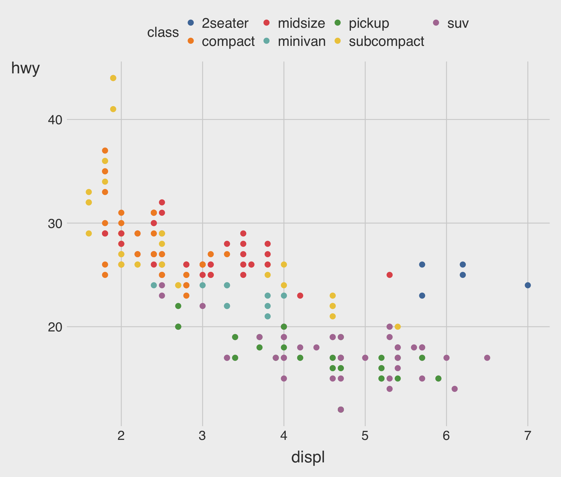
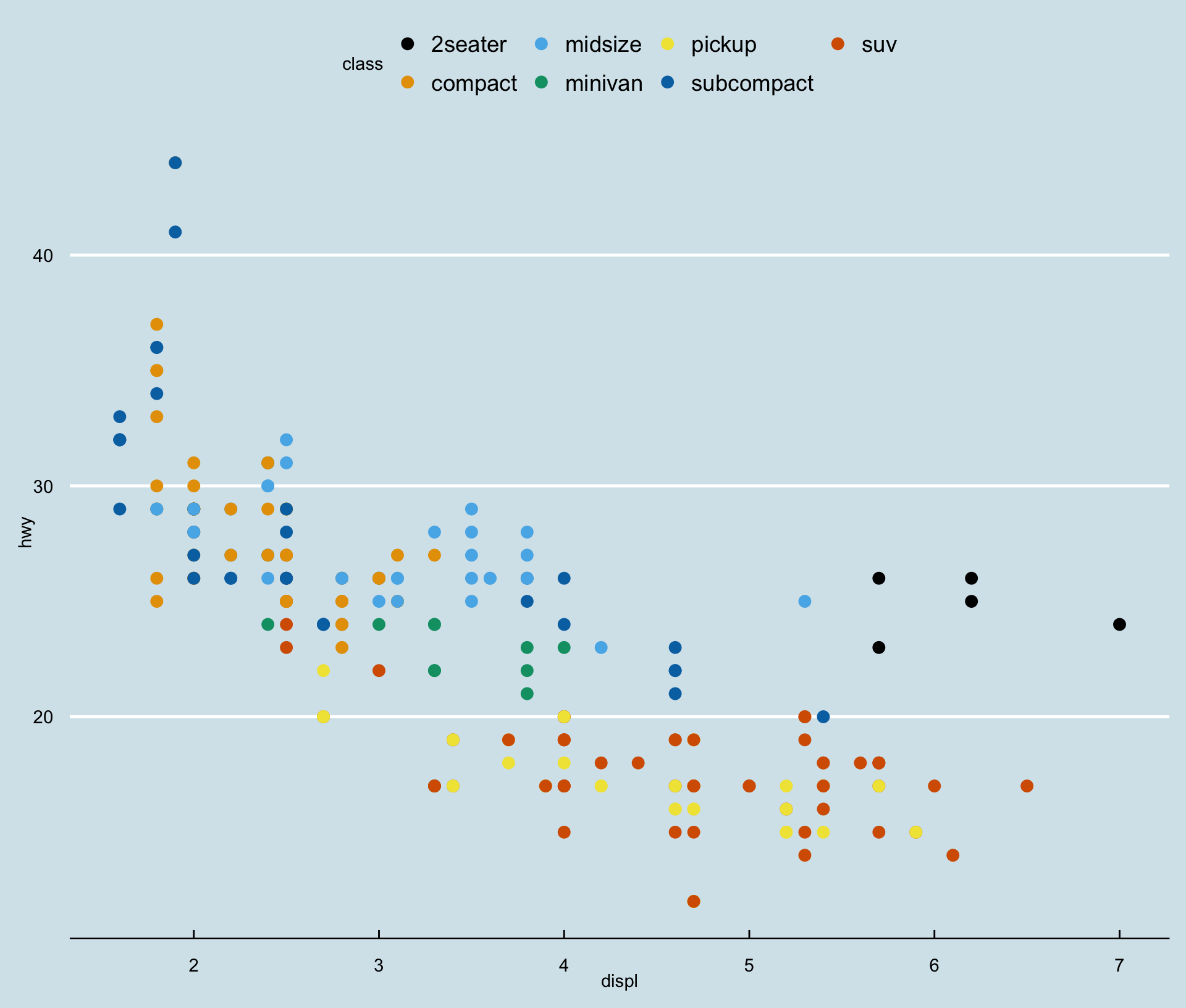
ggthemes::scale_color_colorblind()
- When mapping
colorinaes(), we can usescale_color_*()
ggthemes::scale_color_tableau()
scale_color_tableau()provides color palettes used in Tableau.
💡 Quick Detour
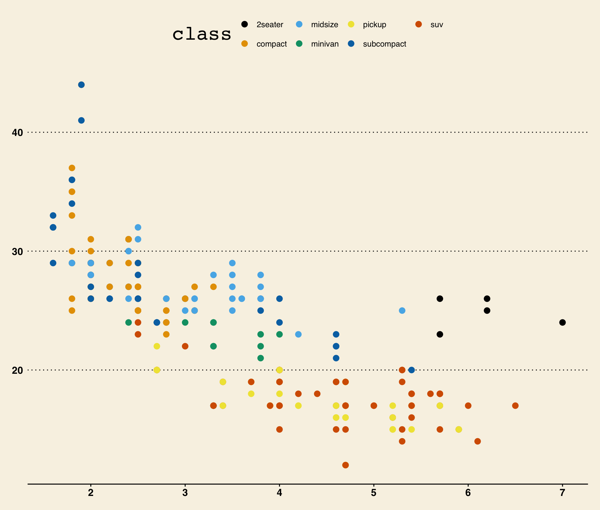
ggthemes::theme_economist()
theme_economist()approximates the style of The Economist.
💡 Quick Detour
ggthemes::theme_wsj()
theme_wsj()approximates the style of The Wall Street Journal.
Boxplots
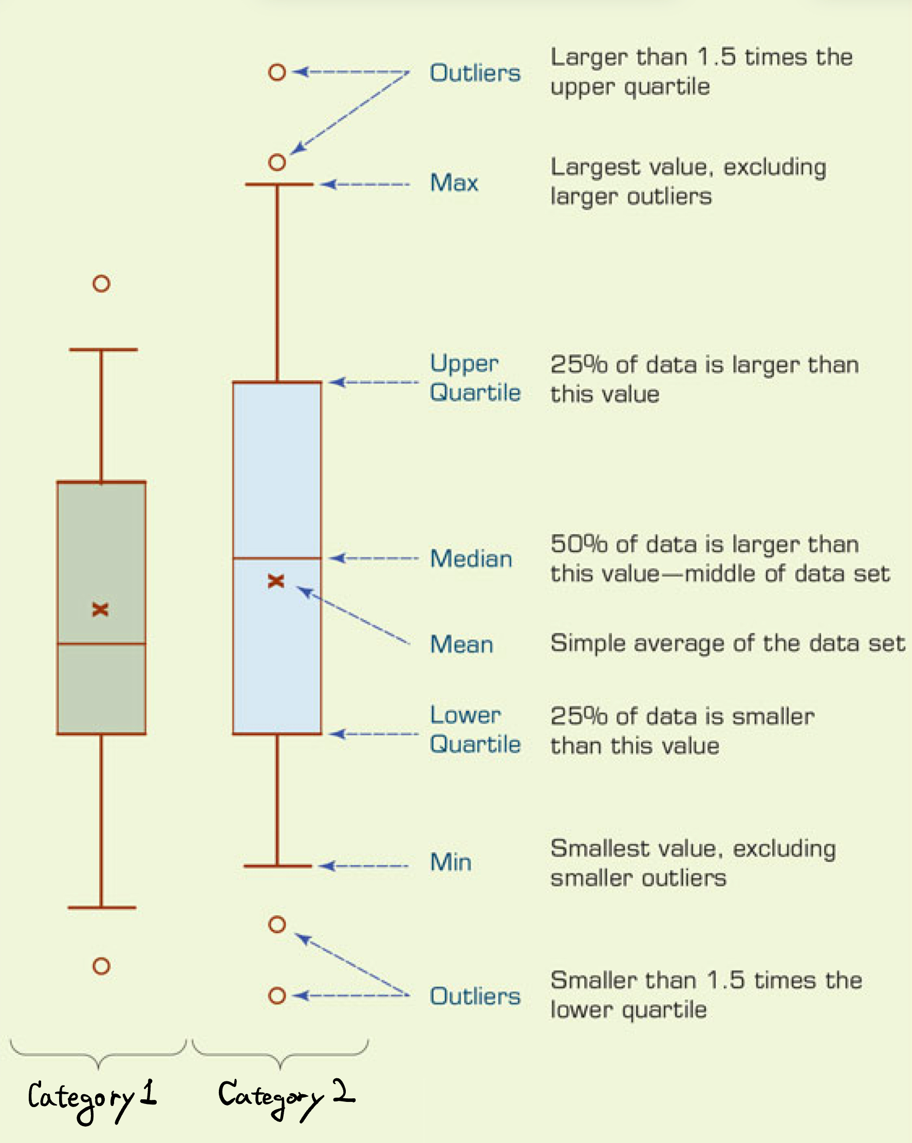
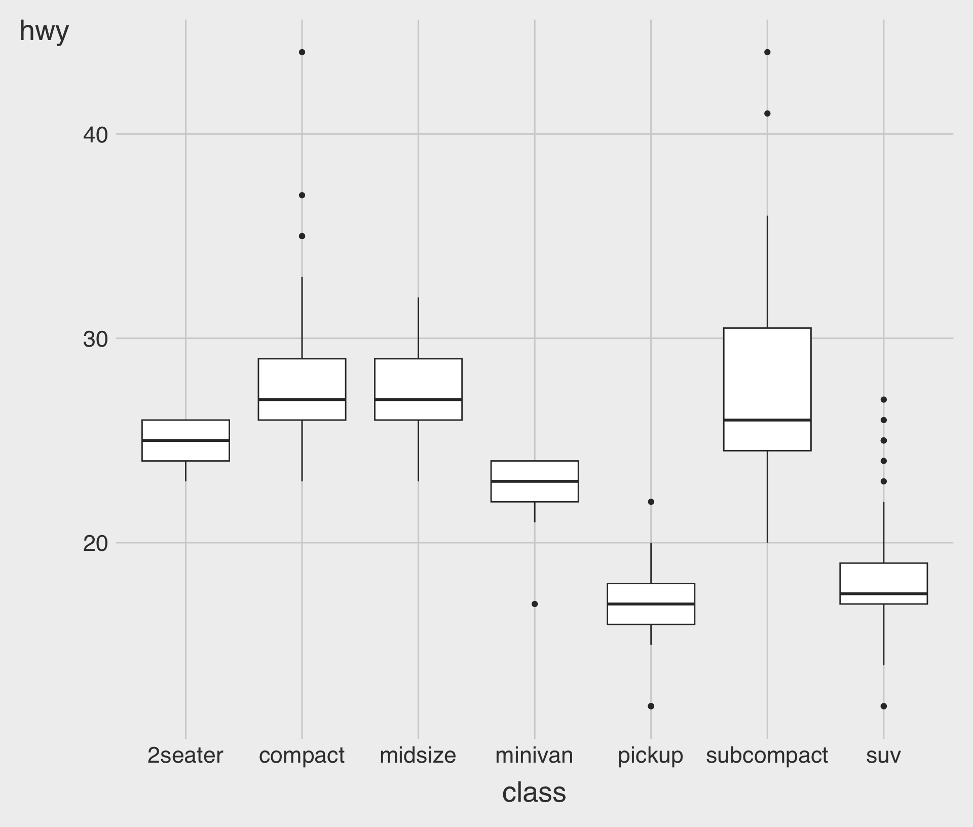
- Boxplots visualize how the distribution of a numeric variable varies across levels of a categorical variable.
- They display the median, quartiles, and potential outliers, providing a compact summary of the data.
Boxplots with geom_boxplot()
geom_boxplot()creates a boxplot;- Mappings: one numeric variable and one categorical variable to the
xandyaesthetics
- Mappings: one numeric variable and one categorical variable to the
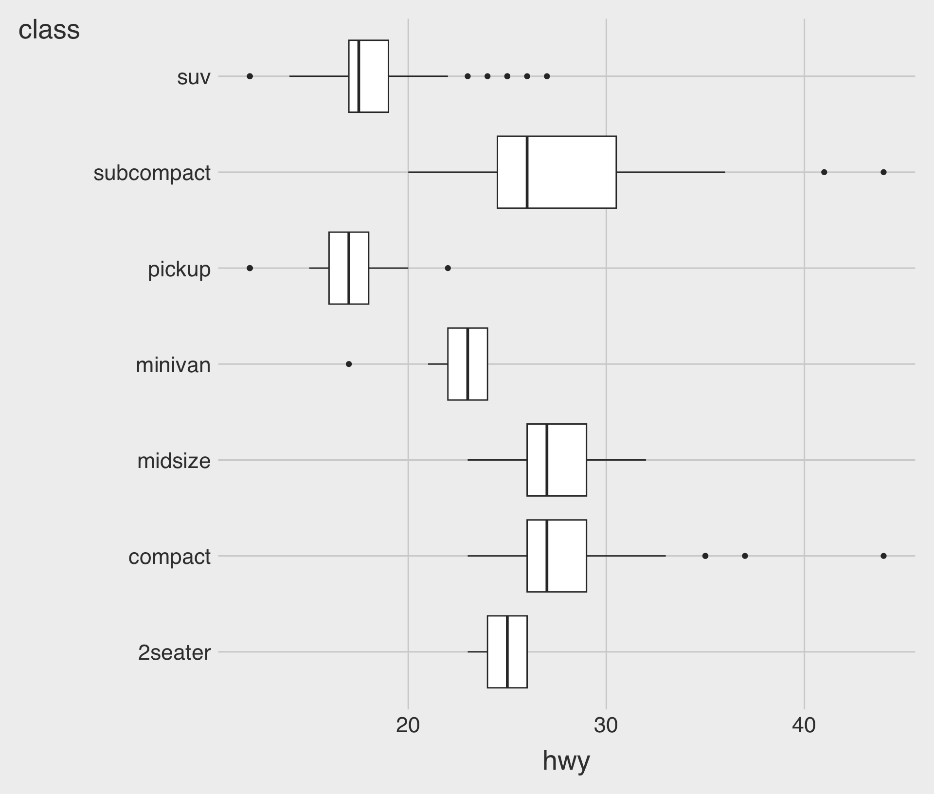
Horizontal Boxplots
- Boxplots can be displayed horizontally or vertically.
- A horizontal boxplot works well when category names are long.
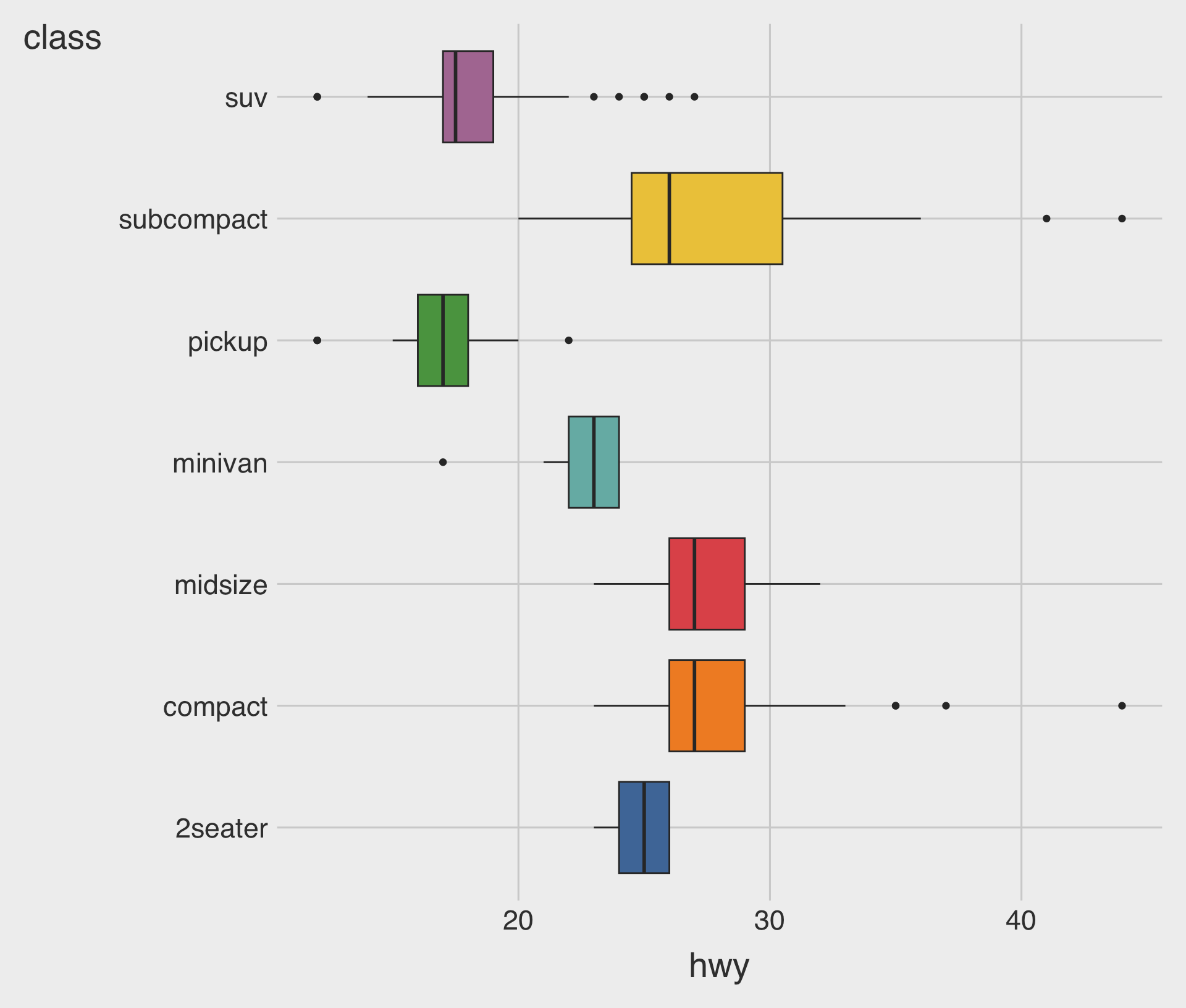
Customizing the fill Aesthetic
# 1. `show.legend = FALSE` turns off
#     the legend information
# 2. `scale_fill_colorblind()` or
#    `scale_fill_tableau()`
#     applies a color-blind friendly
#     palette to the `fill` aesthetic
# install.packages("ggthemes")
library(ggthemes)
ggplot(data = mpg,
       mapping =
         aes(x = hwy,
             y = class,
             fill = class)) +
  geom_boxplot(
    show.legend = FALSE) +
scale_fill_tableau() 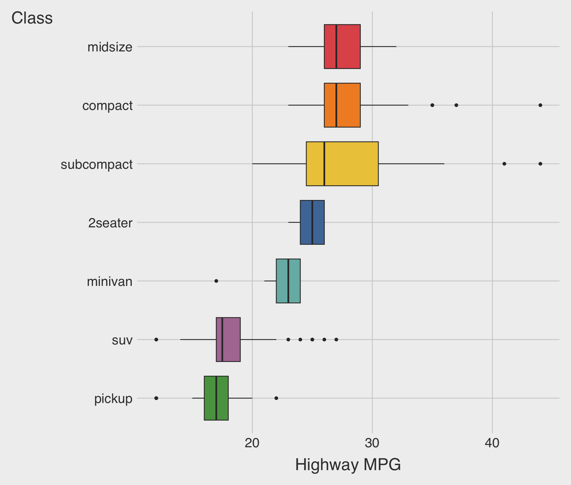
fill: Maps a variable to the fill colors used in the boxplot.ggthemes::scale_fill_tableau(): A colorblind-friendly Tableau-style palette for thefillaesthetic.
Sorted Boxplots with fct_reorder(CATEGORICAL, NUMERICAL)
fct_reorder(CATEGORICAL, NUMERICAL): Reorders the categories of the CATEGORICAL by the median of the NUMERICAL.
Bar Charts
Bar charts are used to visualize the distribution of a categorical variable.
Bar charts display the count (or proportion) of observations for each category.

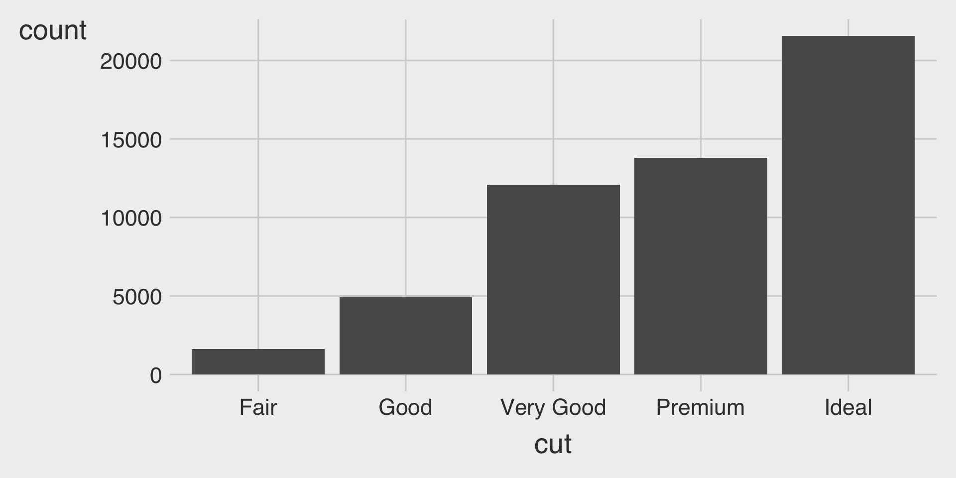
Bar Charts with geom_bar()
geom_bar()creates a bar chart.- We map either the
xoryaesthetic to the variable.
- We map either the
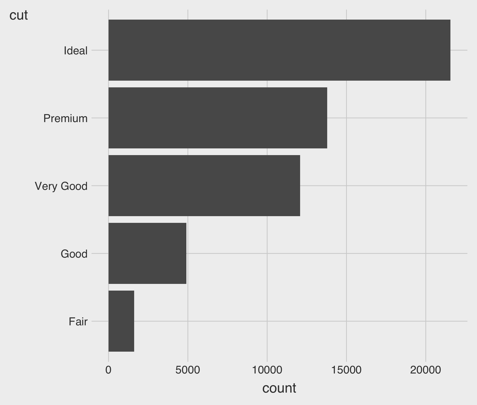
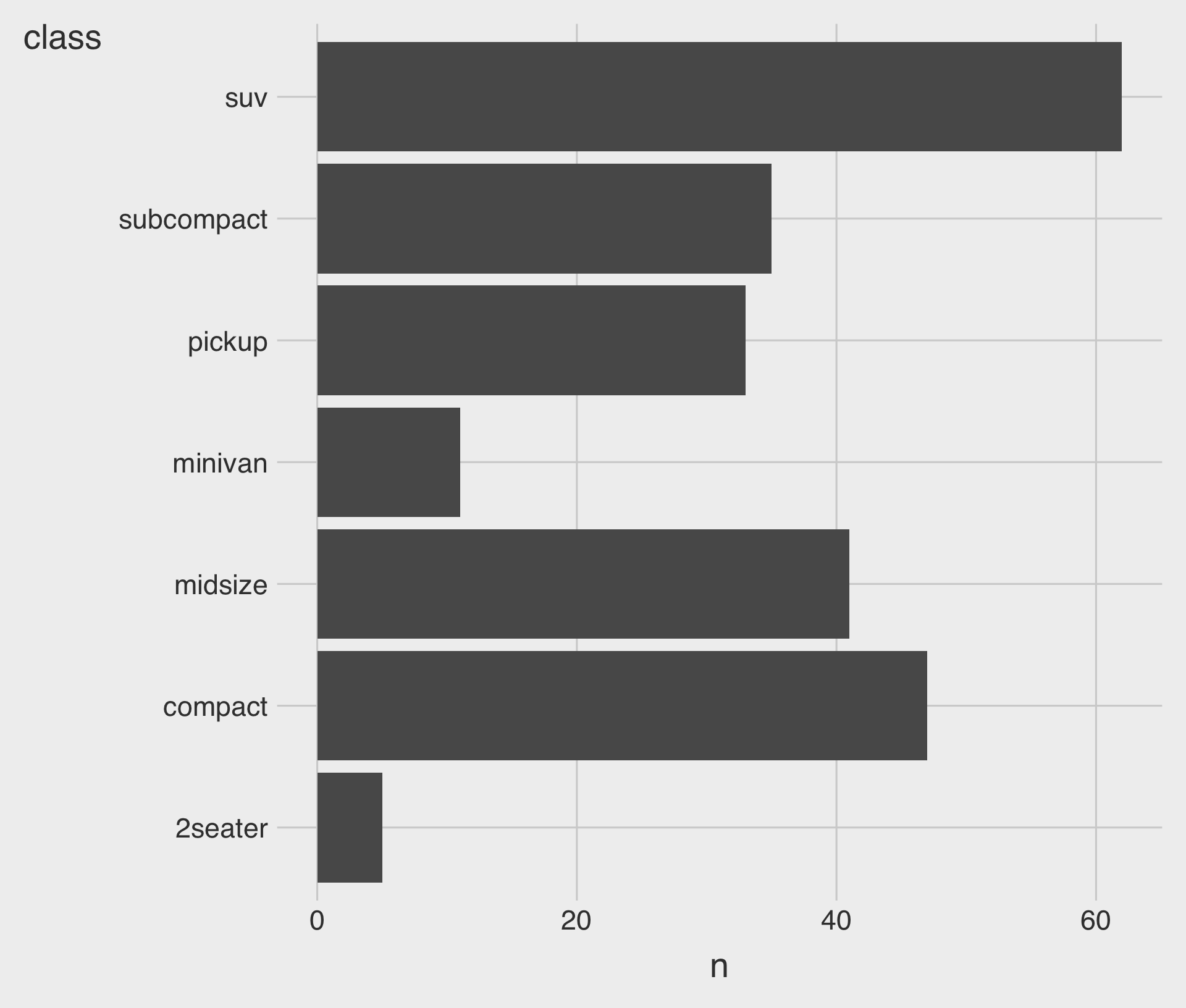
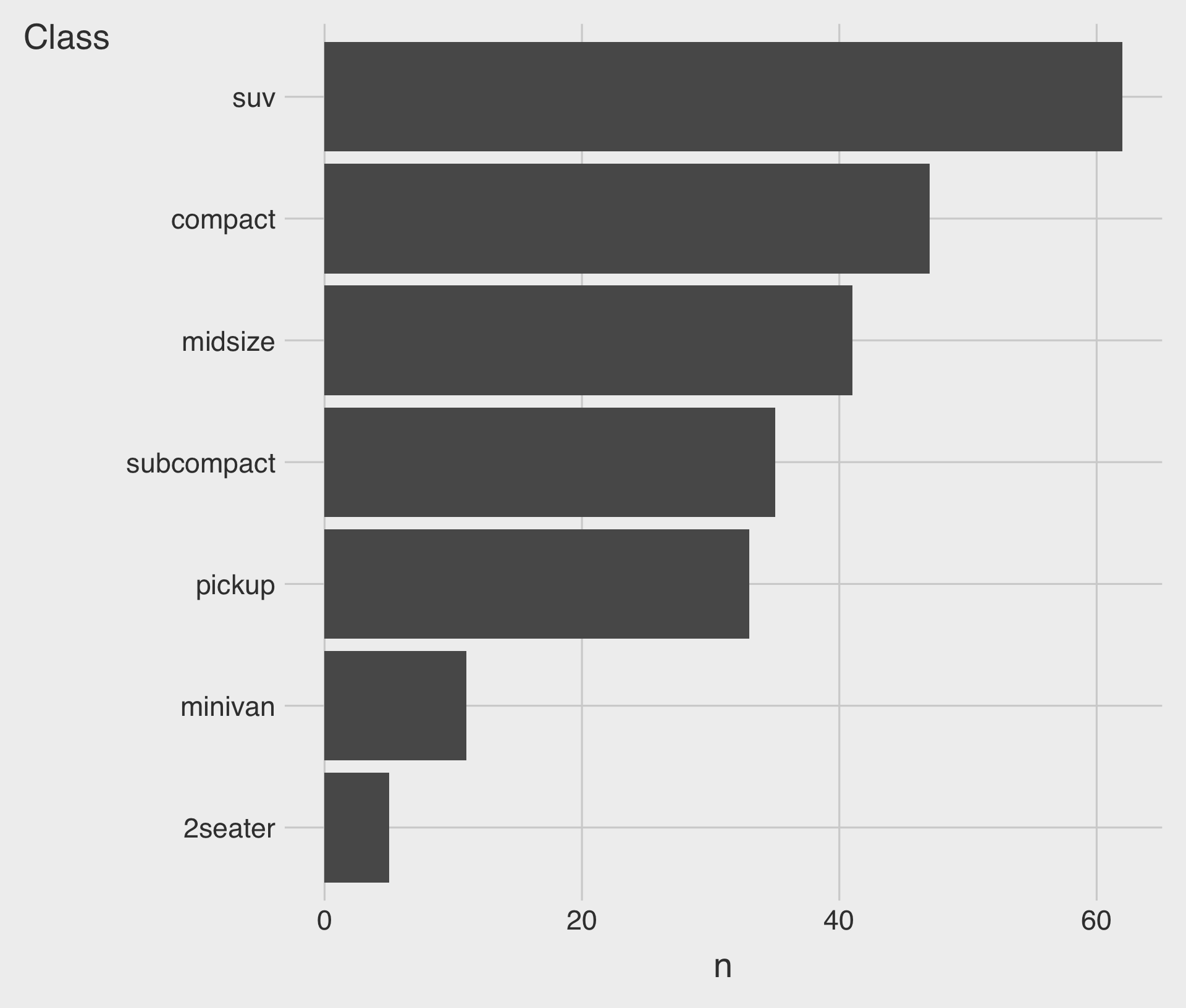
Horizontal Bar Charts
- Bar charts can be horizontal or vertical.
- A horizontal bar chart is a good option for long category names.
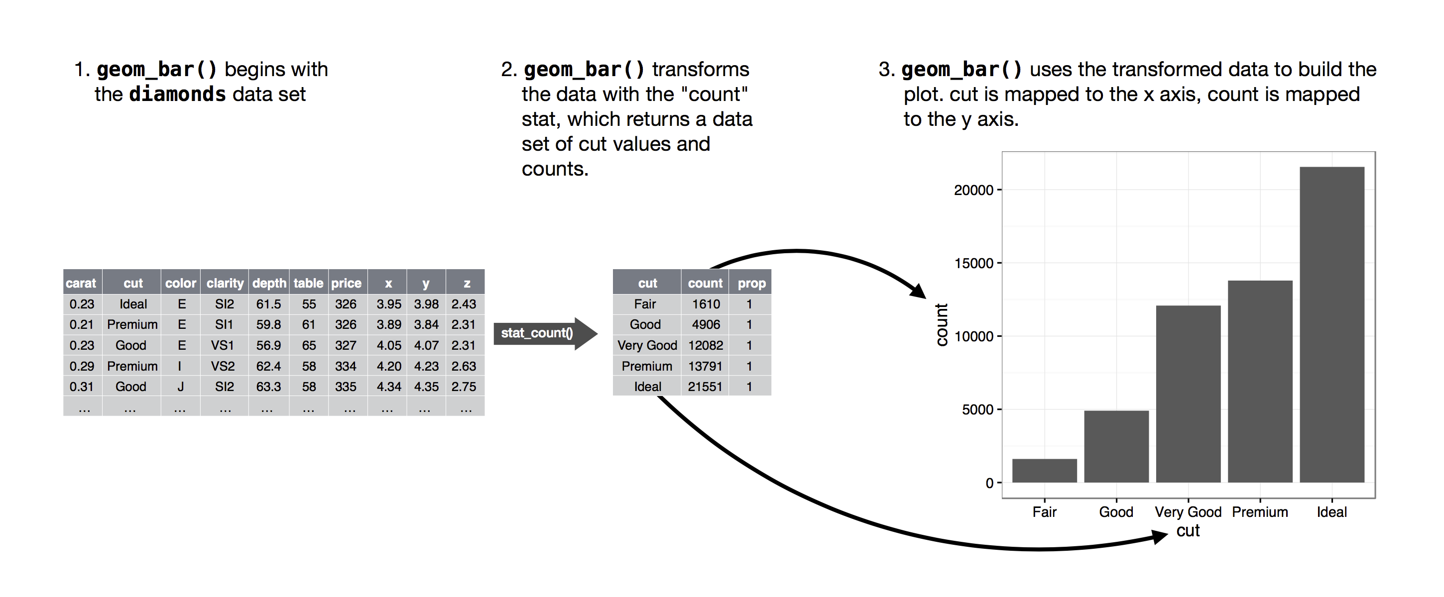
Data Transformation - count(): Counting Occurrences of Each Category in a Categorical Variable
- The figure below demonstrates how the counting process works with
geom_bar().
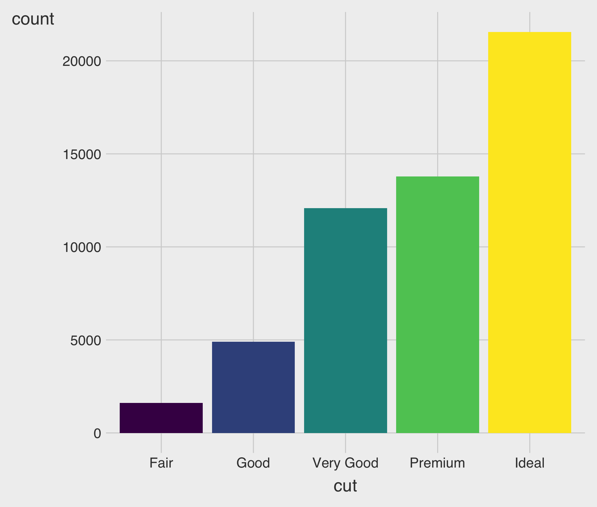
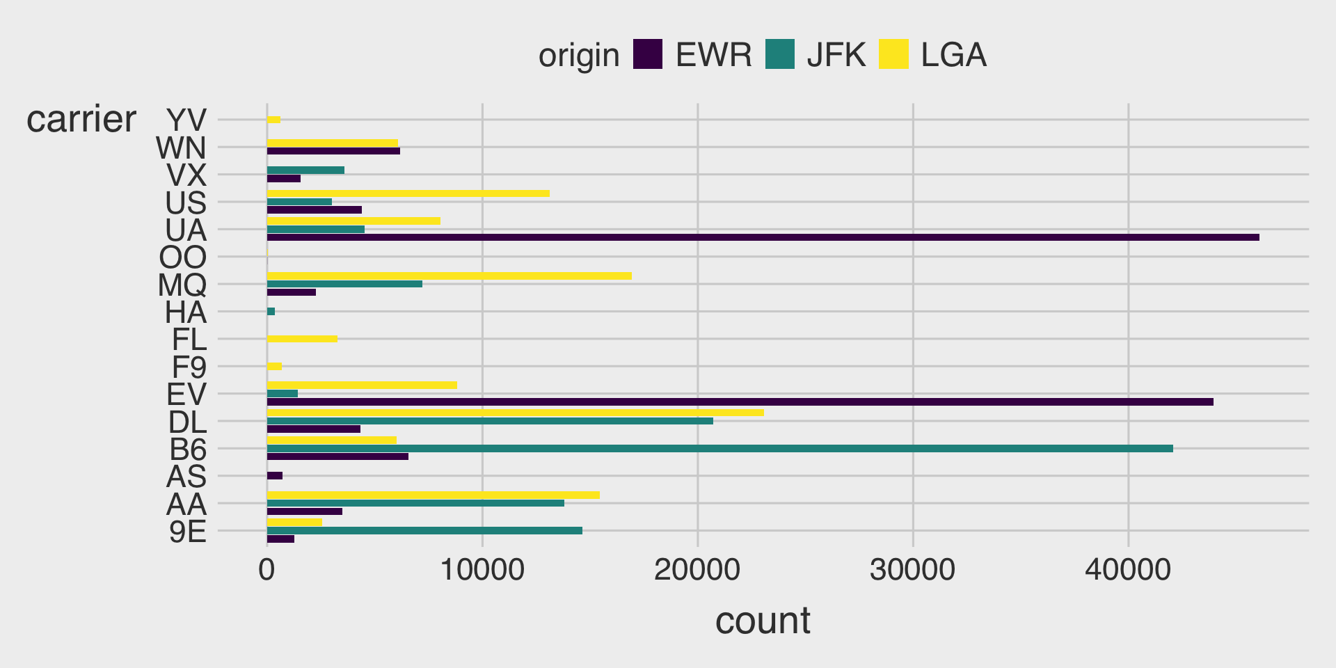
Colorful Bar Charts with the fill Aesthetic

- We can color bar charts using the
fillaesthetic.
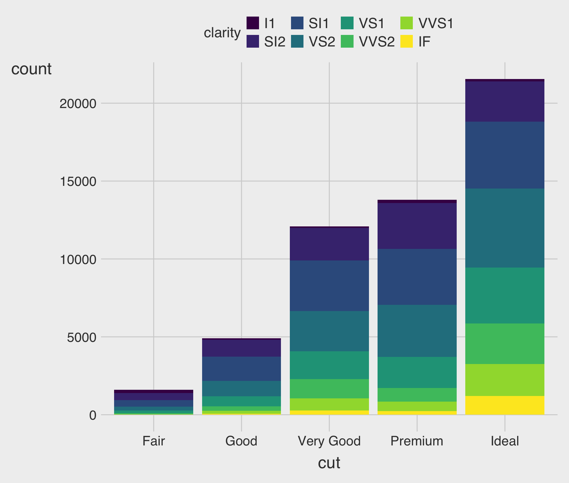
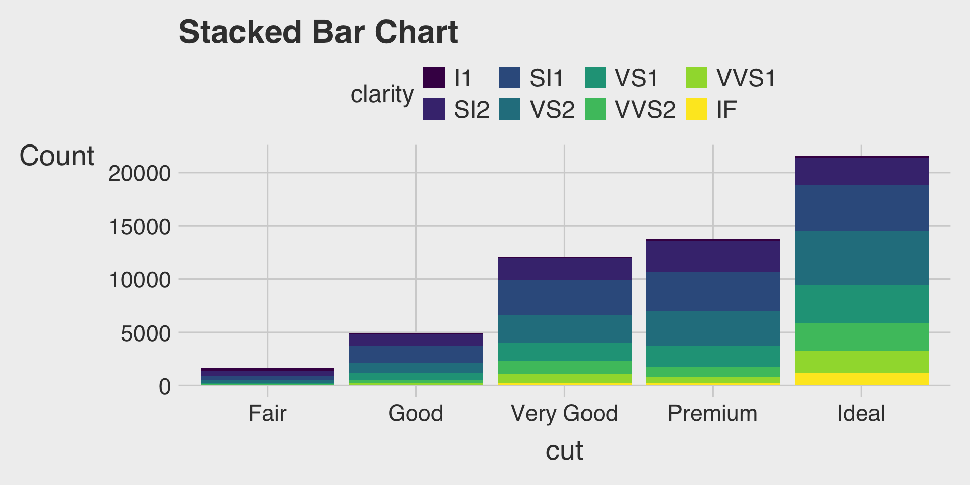
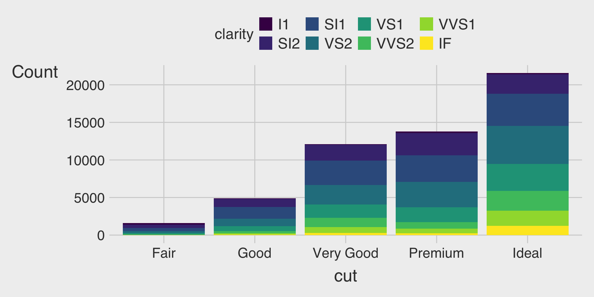
Stacked Bar Charts with the fill Aesthetic
- This describes how the distribution of
clarityvaries bycut, with total bar height for overall count and segments for eachclaritylevel.
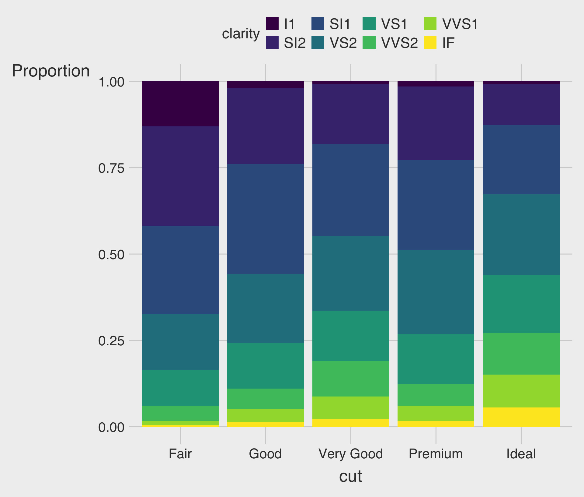
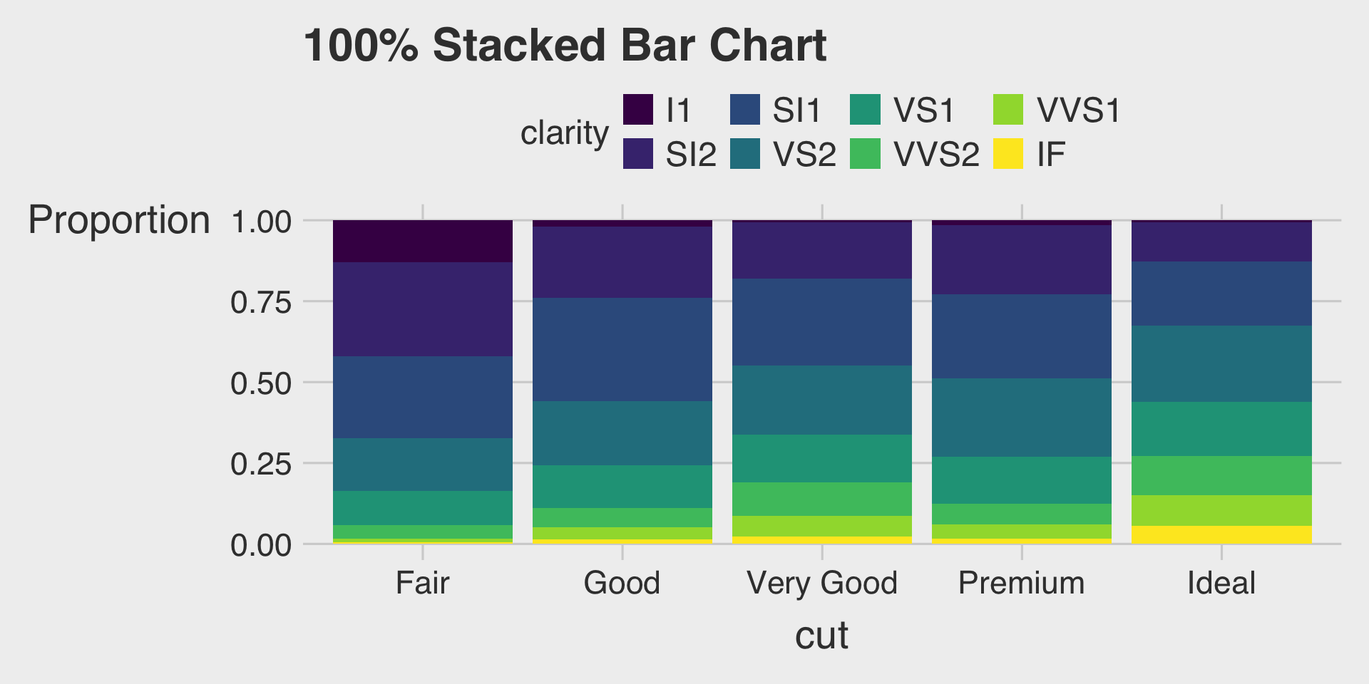
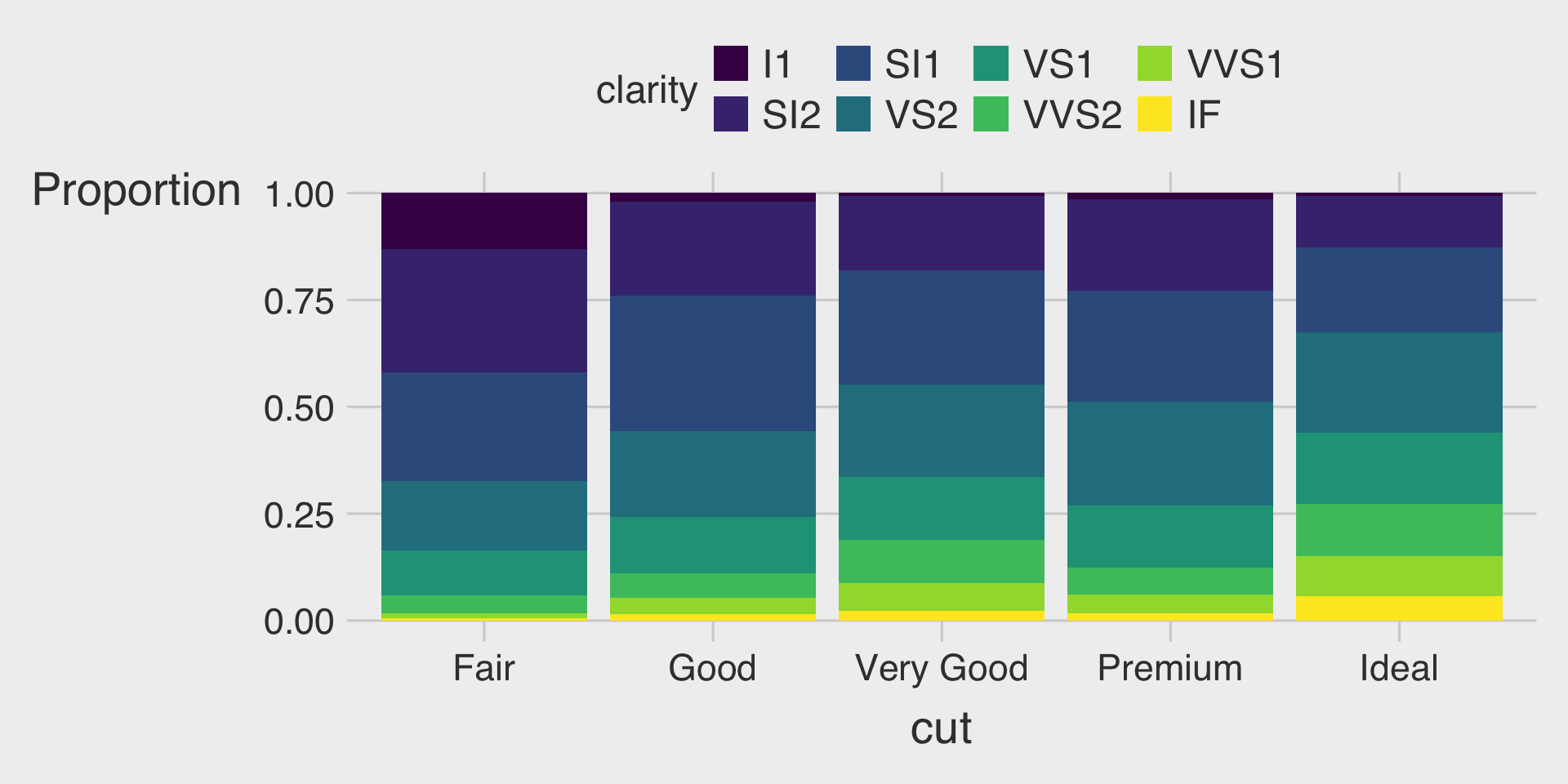
100% Stacked Bar Charts with the fill Aesthetic & position="fill"
- This describes how the distribution of
clarityvaries bycut, displaying the proportion of eachclaritywithin eachcut.
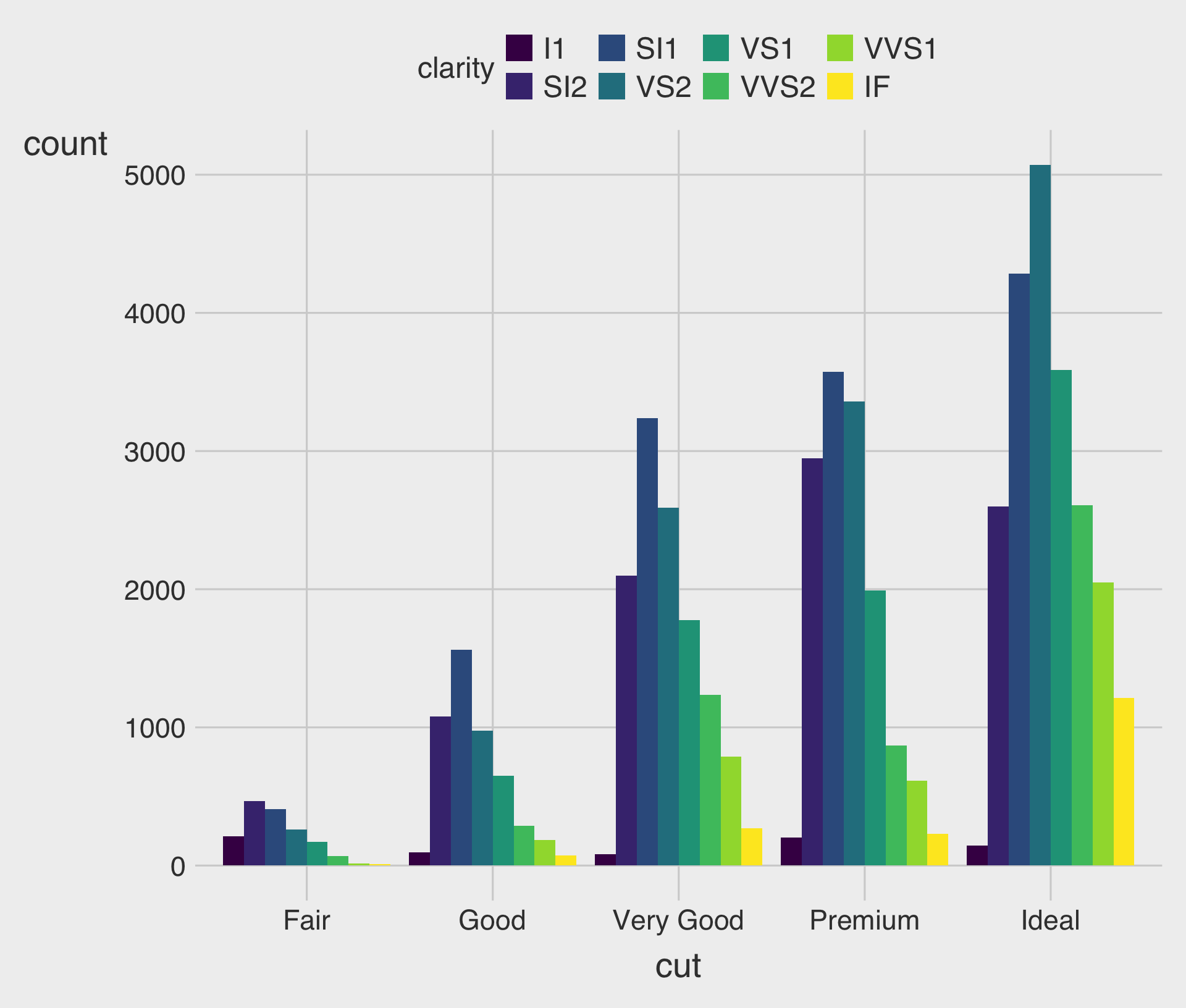
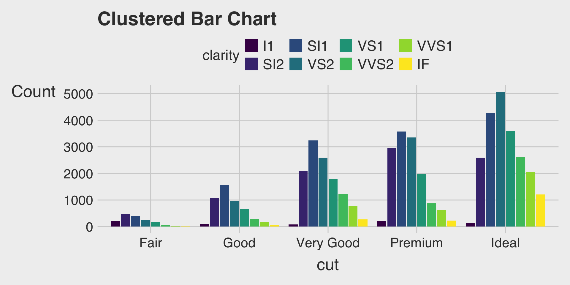
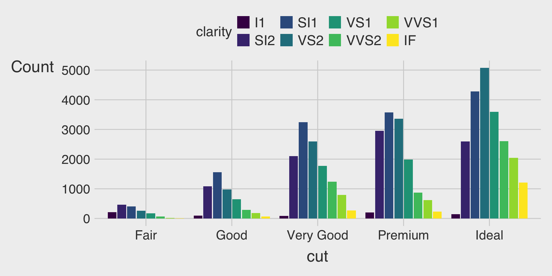
Clustered Bar Charts with the fill Aesthetic & position="dodge"
- This shows how the distribution of
clarityvaries bycut, with separate bars for eachclaritylevel within eachcutcategory.
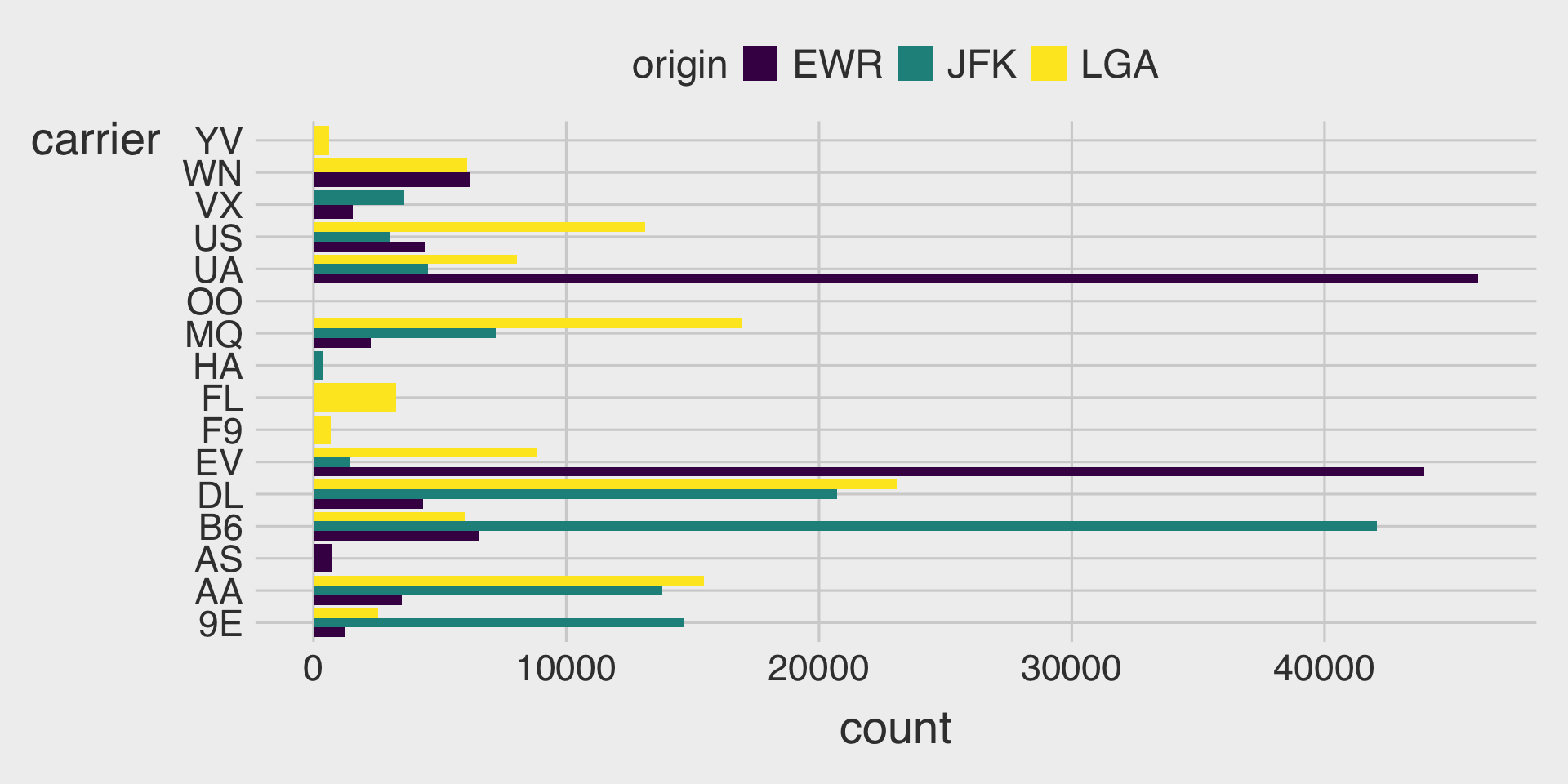
Clustered Bar Charts with the fill Aesthetic & position_dodge2(preserve = "single")
position_dodge2()is useful when some groups have missing categories and you want spacing between bars.
Stacked Bar Charts using the fill Aesthetic and position = "stack"
- The default
positionoption isposition = "stack"
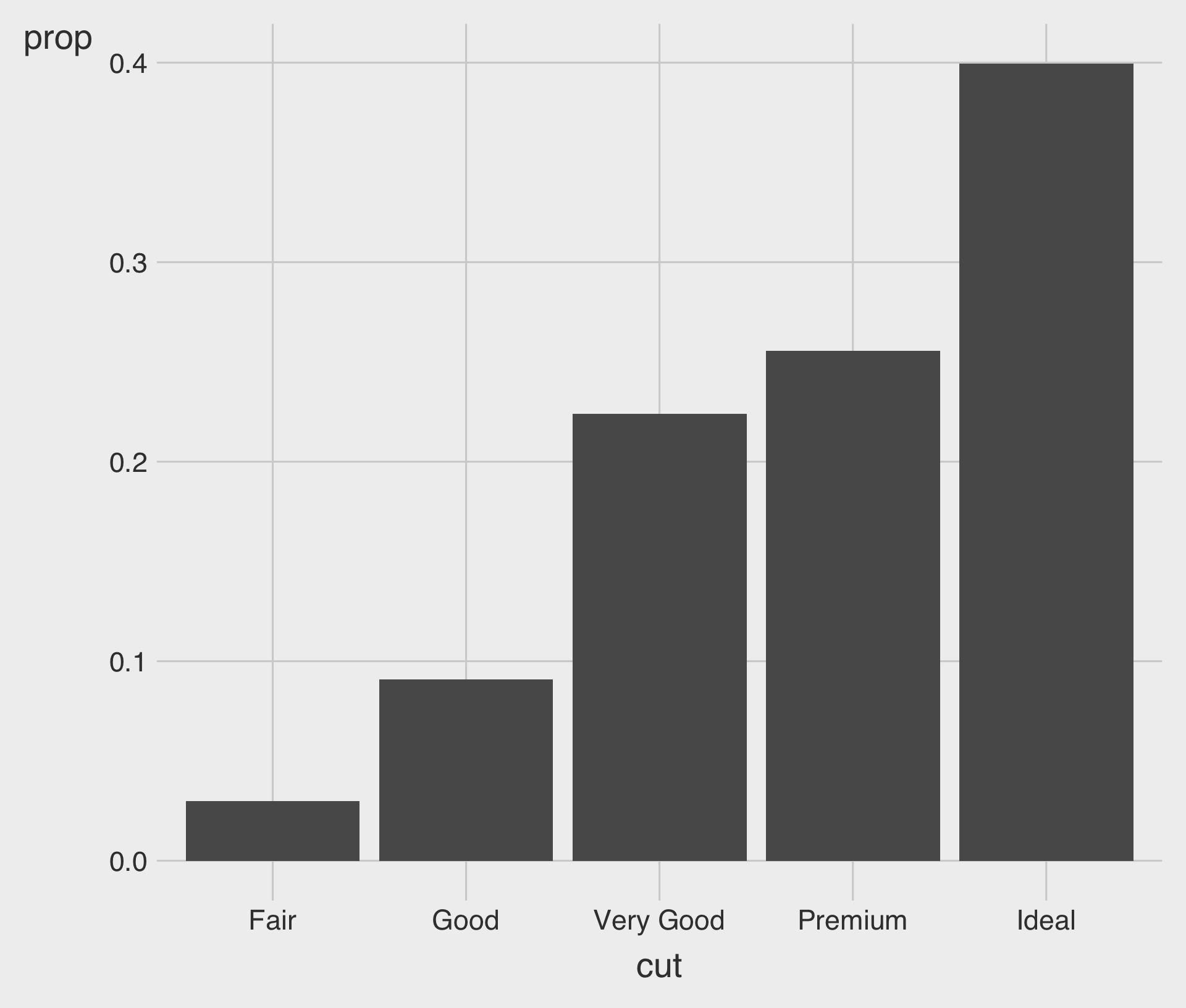
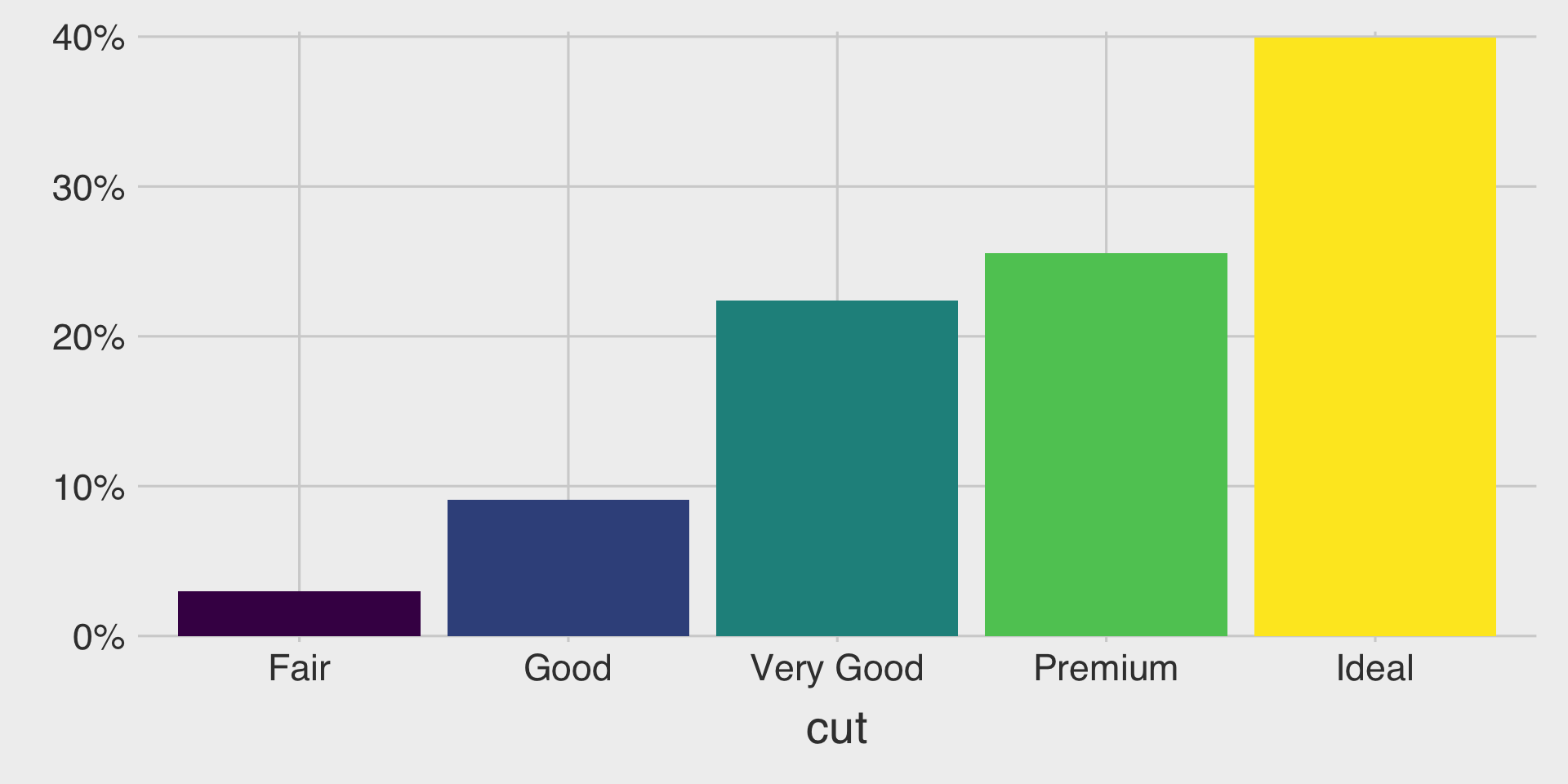
Proportion Bar Charts with geom_bar()
after_stat(prop): Calculates the proportion of the total count.group = 1: Ensures the proportions are calculated over the entire data.frame, not within each group ofcut
Bar Charts with geom_col()
geom_col()creates bar charts where the height of bars directly represents values in acolumn in a given data.frame.geom_col()requires bothx- andy- aesthetics.
Sorted Bar Charts with fct_reorder(CATEGORICAL, NUMERICAL)
fct_reorder(CATEGORICAL, NUMERICAL): Reorders the categories of the CATEGORICAL by the median of the NUMERICAL.
Choosing the Right Bar Charts for Comparing Components and Totals
Which type of bar chart is most effective for your data?
Which type of bar chart best meets your visualization goals?
Stacked Bar Charts
- Purpose: Show the composition of each category while still conveying the overall total.
- When to use: Your primary focus is the total bar height, with a secondary interest in how subcomponents contribute.
- Be cautious: Precise comparisons across subcomponents are difficult because segments do not share a common baseline.
- Tip: If you need to emphasize totals plus composition, a stacked bar chart is a strong choice.
100% Stacked Bar Charts
- Purpose: Display the proportional composition of each category by normalizing all bars to the same height.
- When to use: Your focus is on comparing relative percentages across categories rather than absolute totals.
- Be cautious: While proportions are clear, absolute sizes or totals are not visible.
- Tip: Choose a 100% stacked bar chart when you want to emphasize proportional differences across categories.
Clustered Bar Charts
- Purpose: Plot each subcomponent as a separate bar within each category for side-by-side comparison.
- When to use: Your focus is on comparing individual subcomponents across categories.
- Be cautious: Can become crowded with many categories or subcomponents.
- Tip: Choose a clustered bar chart when you want to emphasize precise comparisons between subcomponents—both within each cluster and across clusters.
Pie Charts: Alternative to Bar Charts?
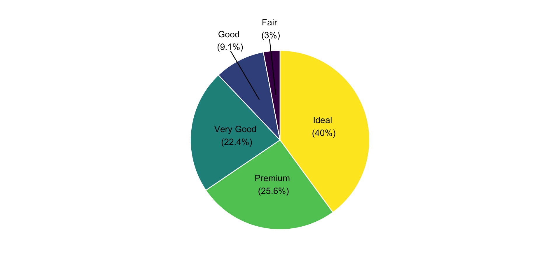
- Pie charts display the proportions of a whole.
- Each slice represents a part of the total.
- But is a pie chart an effective alternative to a bar chart?
- Each slice represents a part of the total.
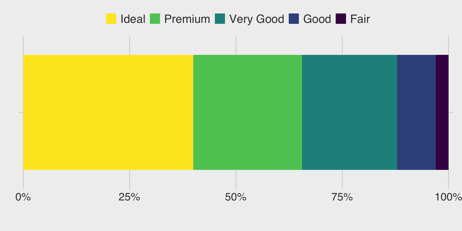
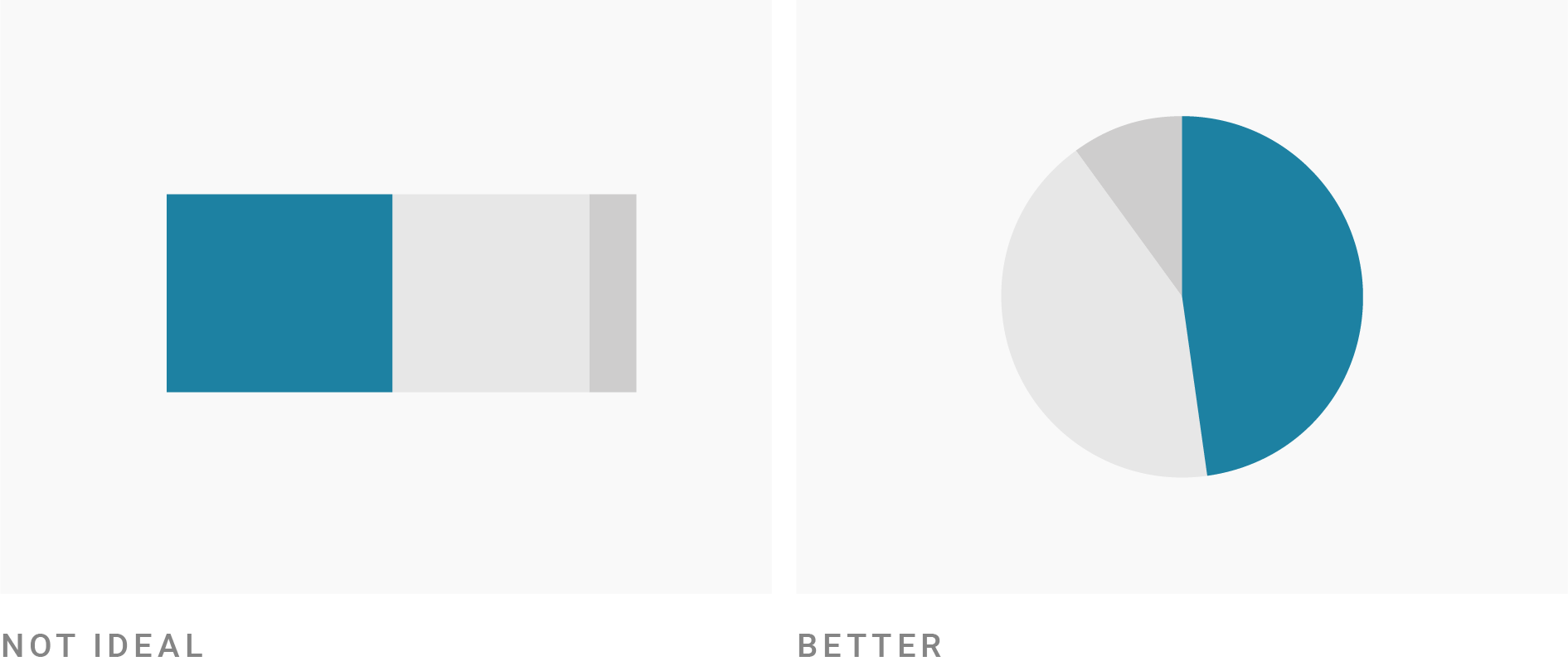
Pie Charts: Alternative to Bar Charts?
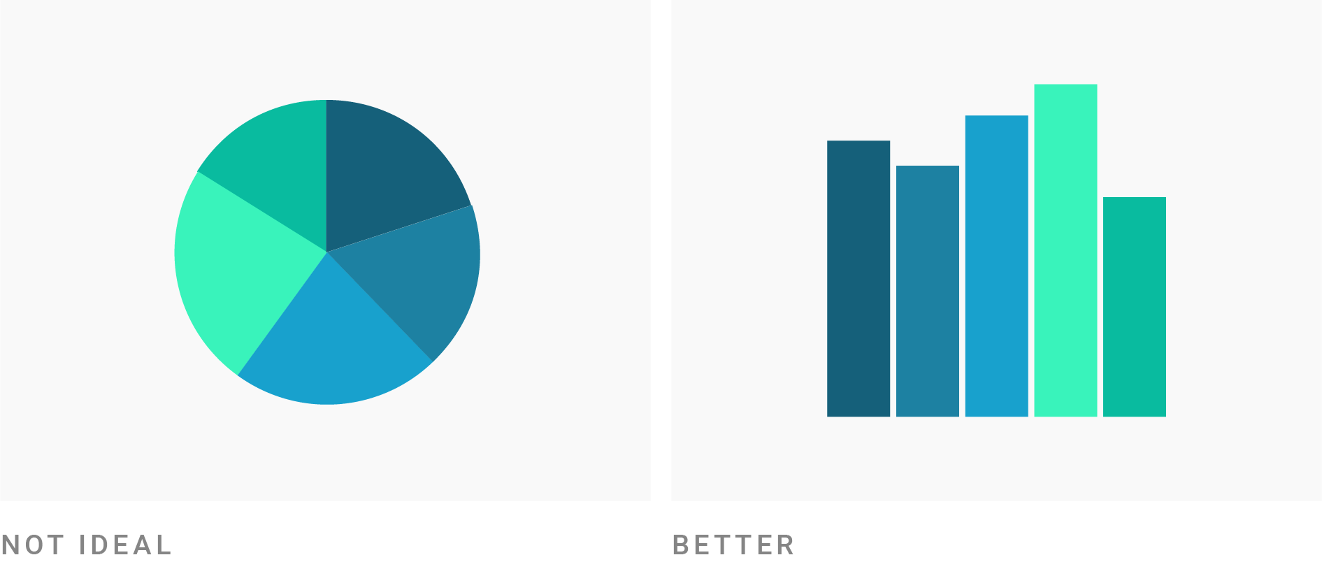
Humans are generally better at judging lengths than angles.
- Still, pie charts can be useful in certain cases.
- Pie charts work best when there are very few categories—ideally four or fewer.
- Pie charts are effective when the goal is to highlight simple, recognizable fractions (e.g., 25%, 50%, 75%).
Pie Charts: Alternative to Bar Charts?
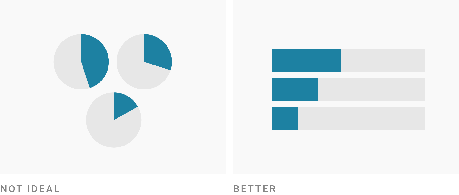
- Pie charts are not ideal when the audience needs to compare the size of individual shares across categories.
- Pie charts are not ideal when the goal is to compare the overall distribution of categories.
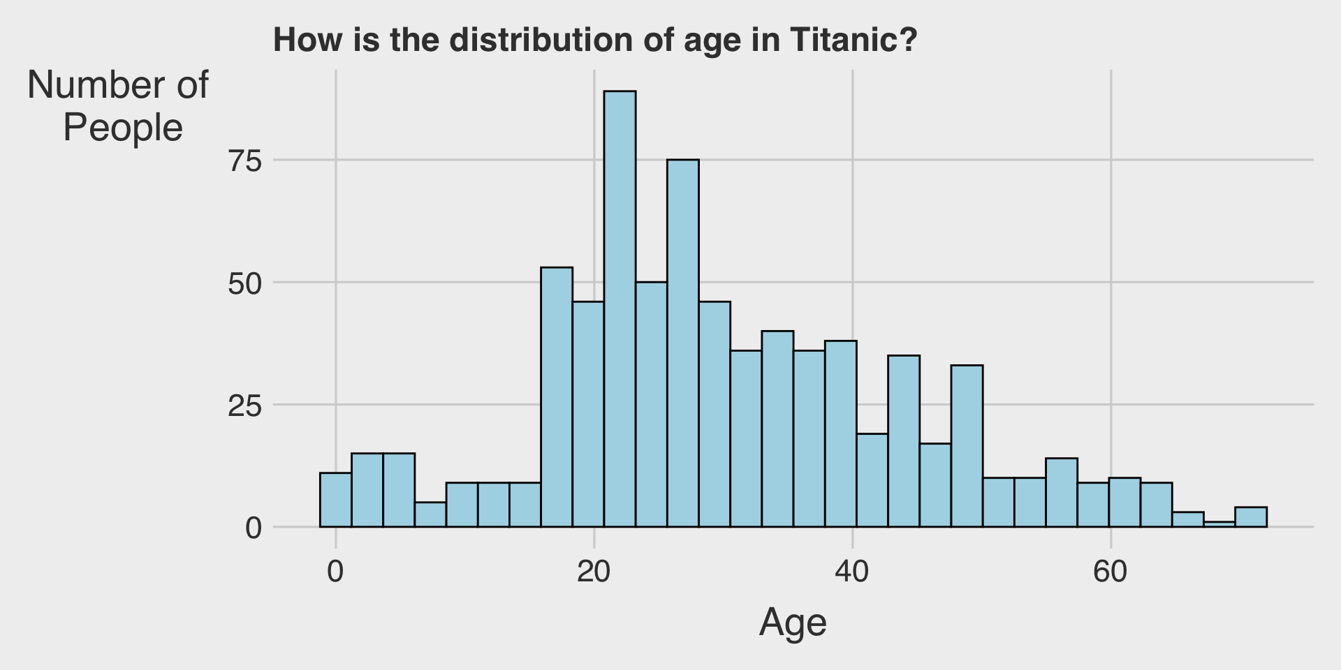
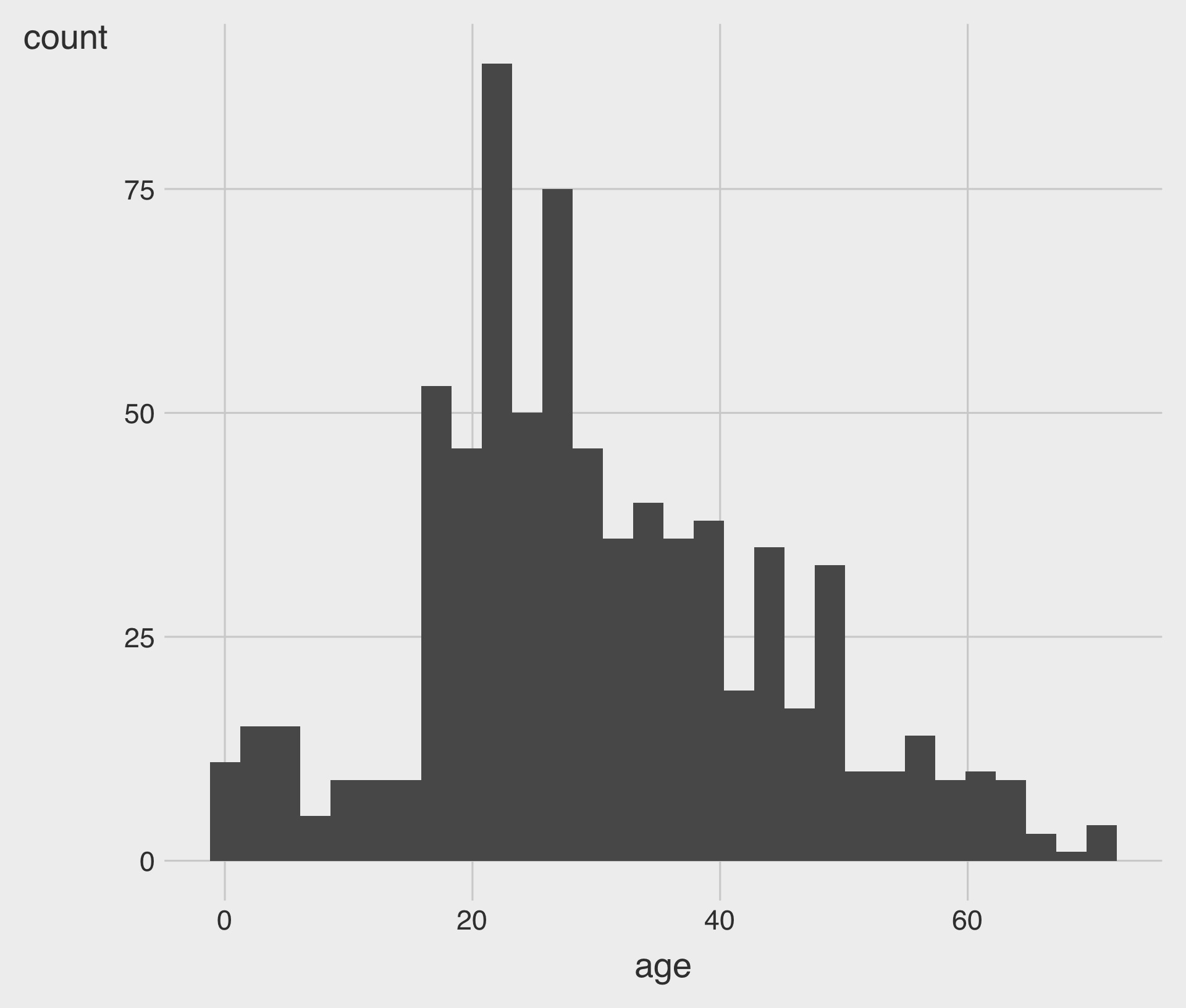
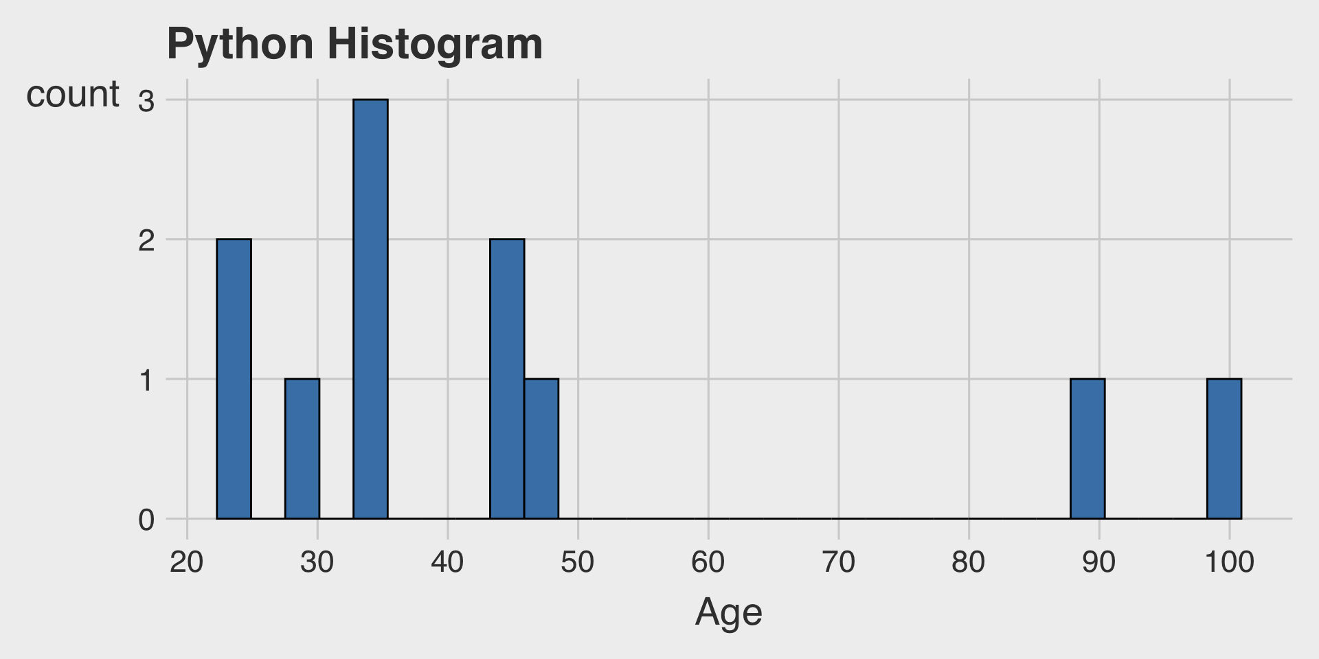
Historams or Bar Charts?
Histograms for the Age variable
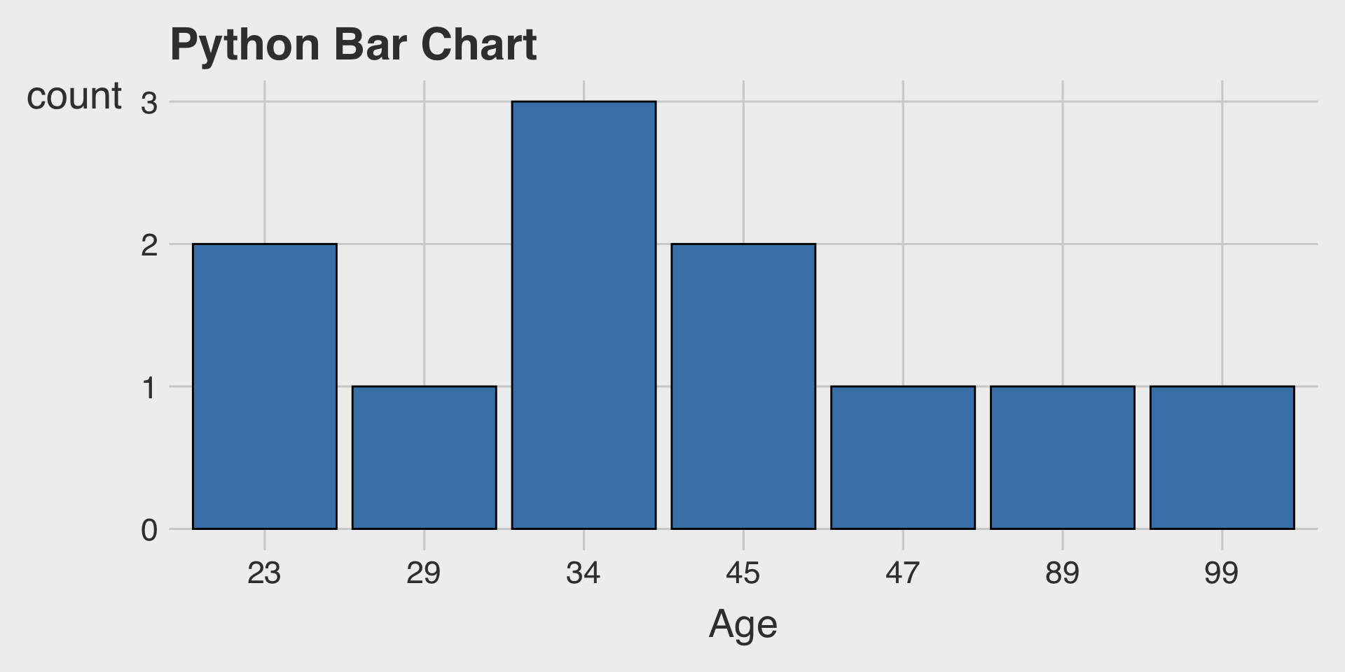
Bar Charts for the Age variable

In ggplot, the distribution of an integer variable can look quite similar whether using
geom_histogram()orgeom_bar().As shown above, in Python and other tools, these visualizations can behave differently, leading to noticeably different outputs.