# install.packages("ggthemes")
library(ggthemes)
library(tidyverse)

flights <- nycflights13::flightsClasswork 5
Distribution Plots and Counting
R Packages
For Classwork 5, please load the following R packages and create the data.frame nycflights13::flights:
Question 1
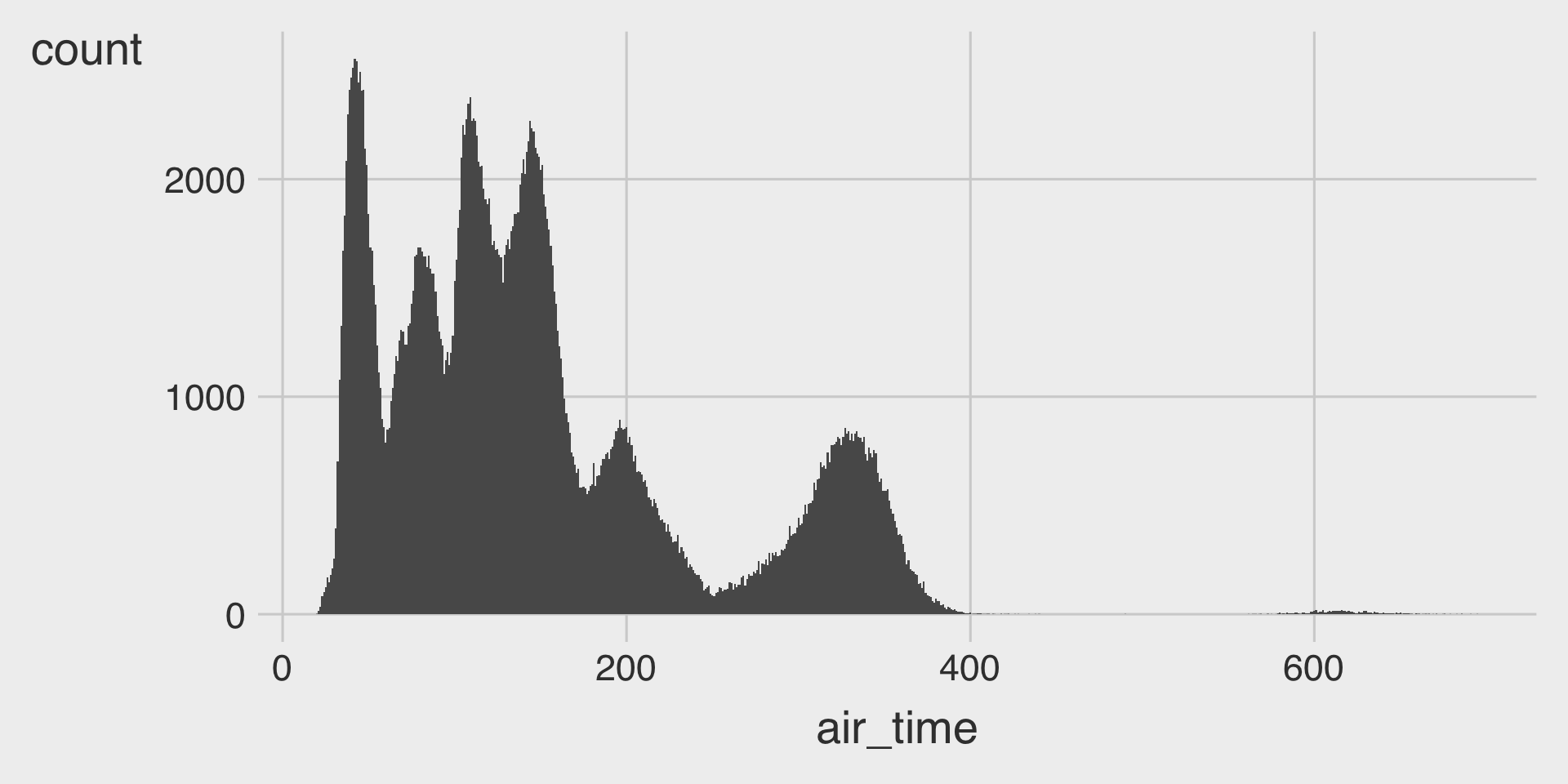
🤖 Task: Fill in the blanks in the provided ggplot() code chunk to visualize the distribution of air_time (minutes spent in the air).
ggplot(data = flights,
       mapping = aes(__BLANK_1__)) +
  geom___BLANK_2__(__BLANK_3__ = 1)
Show answer
ggplot(data = flights,
       mapping = aes(x = air_time)) +
  geom_histogram(binwidth = 1)
Question 2
🤖 Task: Fill in the blanks in the provided ggplot() code chunk to visualize how the distribution of air_time (minutes spent in the air) varies by origin.
Part A. Histograms
ggplot(data = flights,
       mapping = aes(__BLANK_1__)) +
  geom___BLANK_2__(__BLANK_3__ = 50,
                   __BLANK_4__ = "lightblue") +
  facet_wrap(__BLANK_5__)
Show answer
ggplot(data = flights,
       mapping = aes(x = air_time)) +
  geom_histogram(bins = 50,
                 fill = "lightblue") +
  facet_wrap(~origin)
Part B. Density Plots
ggplot(data = flights,
       mapping = aes(__BLANK_1__,
                     __BLANK_2__ = origin,
                     __BLANK_3__ = origin)) +
  geom__BLANK_4__(__BLANK_5__)
Show answer
ggplot(data = flights,
       mapping = aes(x = air_time,
                     color = origin,
                     fill = origin)) +
  geom_density(alpha = .33)
Part C. Boxplots
ggplot(data = flights,
       mapping = aes(__BLANK_1__,
                     y = __BLANK_2__,
                     __BLANK_3__,
                     )) +
  geom___BLANK_4__(show.legend = FALSE)
Show answer
ggplot(data = flights,
       mapping = aes(x = air_time,
                     y = origin,
                     fill = origin)) +
  geom_boxplot(show.legend = FALSE)
Question 3
🤖 Task: Create the data frame top3_n, containing two variables and five observations:
carrier: the top 3 carriers ranked by number of flights
n: the number of flights operated by each of those carriers
__BLANK_1__ <- flights |>
  __BLANK_2__ |>
  __BLANK_3__( desc(n) ) |>
  head(3)  # returns the first 3 observations in the given data.frame
Show answer
top3_n <- flights |>
  count(carrier) |>
  arrange(-n) |>
  head(3)
Question 4
🤖 Task: Create the data.frame top3_carriers, containing six variables (month, day, dep_time, carrier, origin, and dest) and all observations for flights operated by only the top 3 carriers identified in Question 3.
__BLANK_1__ <- flights |>
  filter(__BLANK_2__) |>
  __BLANK_3__(month, day, dep_time, carrier, origin, dest)
Show answer
top3_carriers <- flights |>
  filter(carrier == "UA" |
         carrier == "B6" |
         carrier == "EV" ) |>
  select(month, day, dep_time, carrier, origin, dest)
Question 5
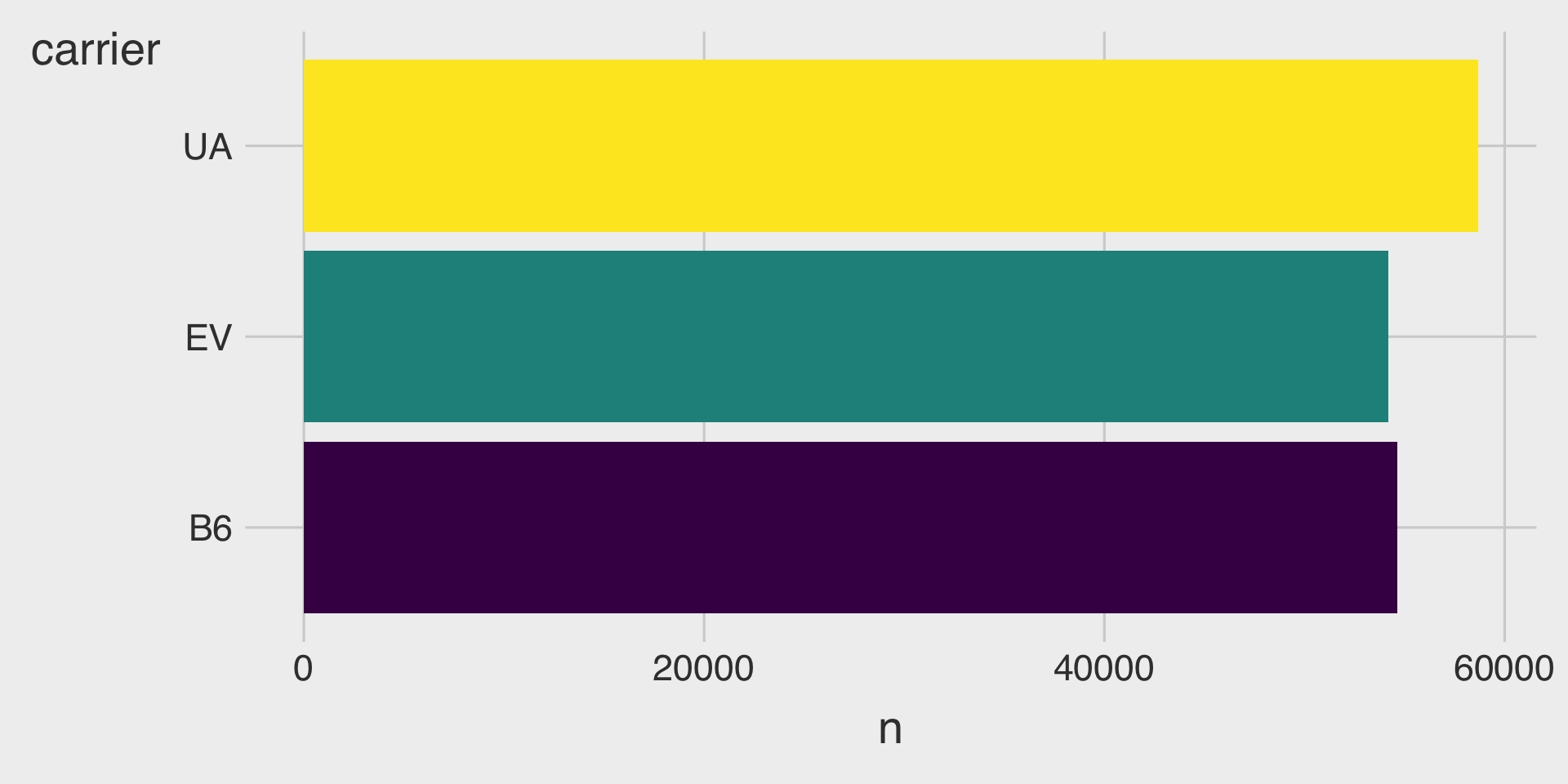
🤖 Task: Fill in the blanks in the provided ggplot() code chunks to visualize the distribution of carrier using the top3_carriers data.frame.
Part A. Bar Charts

ggplot(data = top3_carriers,
       mapping = aes(__BLANK_1__,
                     fill = __BLANK_2__)) +
  geom___BLANK_3__(show.legend = FALSE)
Show answer
ggplot(data = top3_carriers,
       mapping = aes(y = carrier,
                     fill = carrier)) +
  geom_bar(show.legend = FALSE)
Part B. Proportion Bar Charts
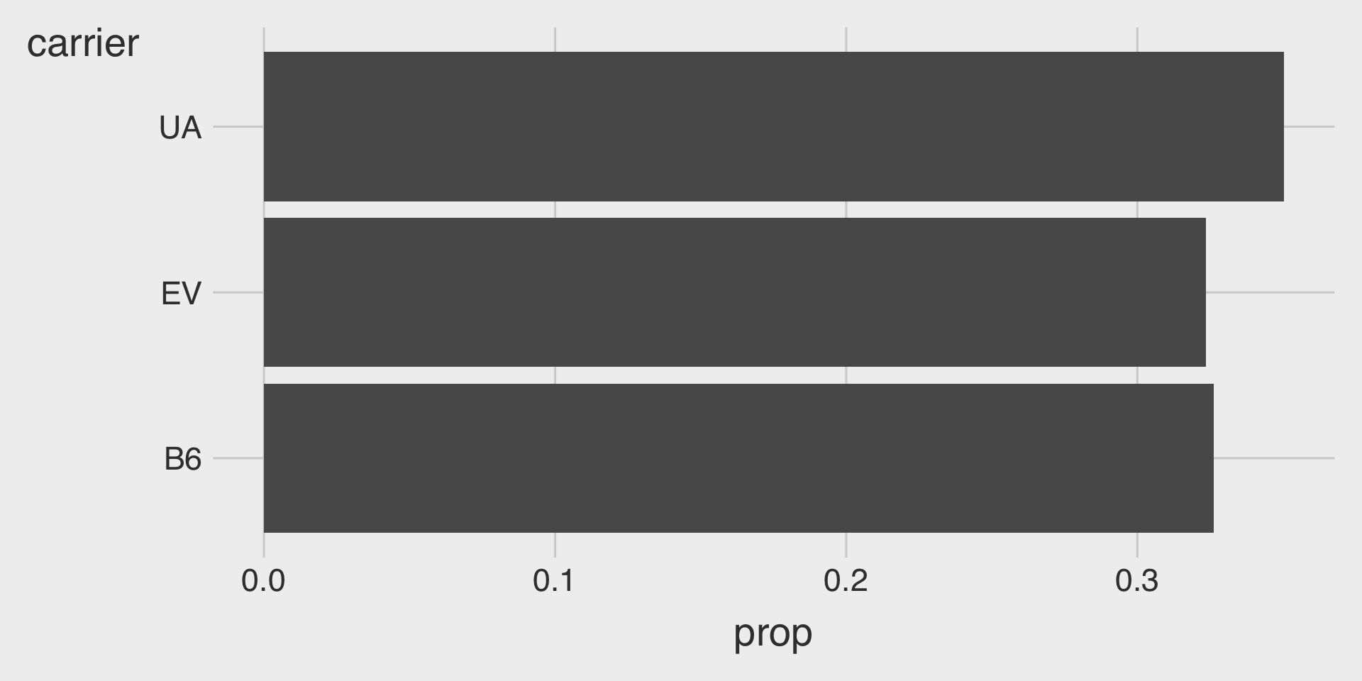
ggplot(data = top3_carriers,
       mapping = aes(__BLANK_1__,
                     x = __BLANK_2__,
                     __BLANK_3__ = 1)) +
  geom___BLANK_4__(show.legend = FALSE)
Show answer
ggplot(data = top3_carriers,
       mapping = aes(y = carrier,
                     x = after_stat(prop),
                     group = 1)) +
  geom_bar(show.legend = FALSE)
Question 6
🤖 Task: Fill in the blanks in the provided ggplot() code chunks to visualize how the distribution of carrier varies by origin using the top3_carriers data.frame.
Part A. Stacked Bar Charts
ggplot(data = __BLANK_1__,
       mapping = aes(y = __BLANK_2__,
                     __BLANK_3__)) +
  geom_bar()
Show answer
ggplot(data = top3_carriers,
       mapping = aes(y = origin,
                     fill = carrier)) +
  geom_bar()
Part B. 100% Stacked Bar Charts
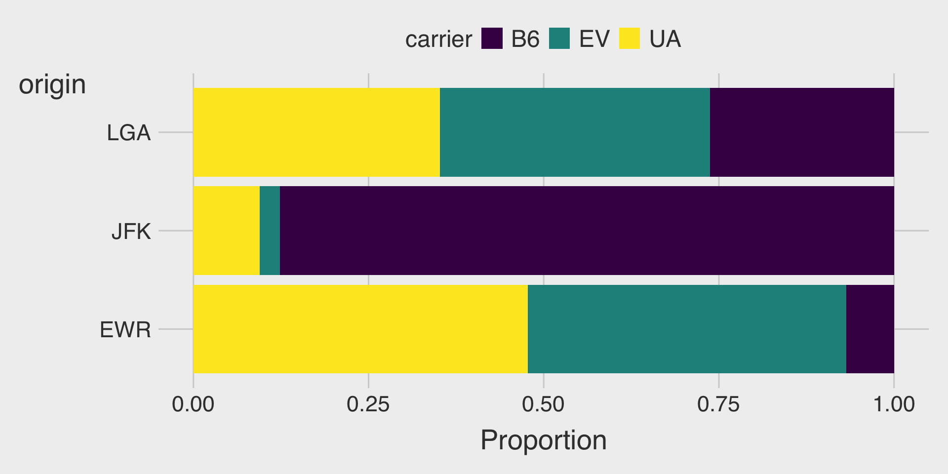
ggplot(data = __BLANK_1__,
       mapping = aes(y = __BLANK_2__,
                     __BLANK_3__)) +
  geom_bar(position = __BLANK_4__) +
  labs(x = "Proportion") # label x-axis title
Show answer
ggplot(data = top3_carriers,
       mapping = aes(y = origin,
                     fill = carrier)) +
  geom_bar(position = "fill") +
  labs(x = "Proportion") # label x-axis title
Part C. Clustered Bar Charts
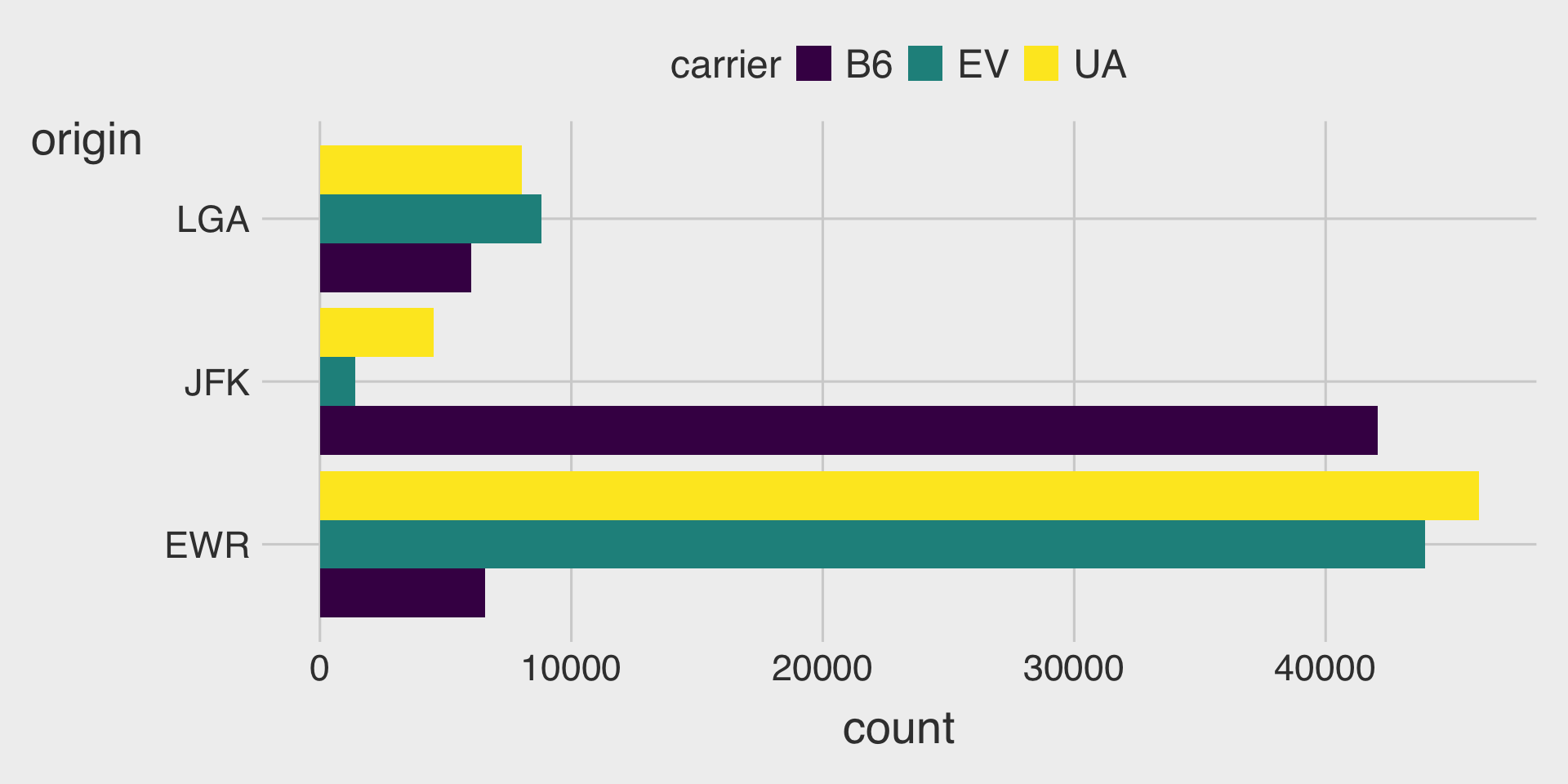
ggplot(data = __BLANK_1__,
       mapping = aes(y = __BLANK_2__,
                     __BLANK_3__)) +
  geom_bar(position = __BLANK_4__)
Show answer
ggplot(data = top3_carriers,
       mapping = aes(y = origin,
                     fill = carrier)) +
  geom_bar(position = "dodge")
Part D. Facetted Bar Charts
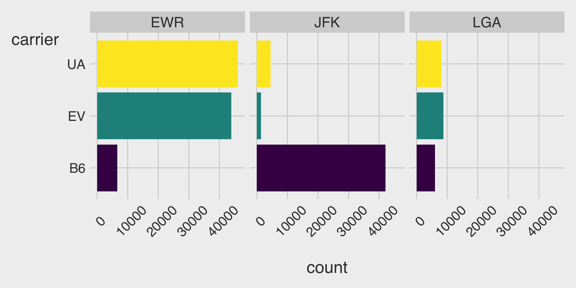
ggplot(data = __BLANK_1__,
       mapping = aes(y = __BLANK_2__,
                     __BLANK_3__)) +
  geom_bar(show.legend = FALSE) +
  facet_wrap(__BLANK_4__)
Show answer
ggplot(data = top3_carriers,
       mapping = aes(y = carrier,
                     fill = carrier)) +
  geom_bar(show.legend = F) +
  facet_wrap(~origin) +
  theme(
    axis.text.x = element_text(angle = 45,
                               margin = margin(20,0,0,0))
    )
Question 7
🤖 Task: Fill in the blanks in the provided ggplot() code chunk to visualize the distribution of carrier using the top3_n data.frame.

ggplot(data = top3_n,
       mapping = aes(x = __BLANK_1__,
                     y = __BLANK_2__,
                     __BLANK_3__)) +
  geom___BLANK_4__(show.legend = FALSE)
Show answer
ggplot(data = top3_n,
       mapping = aes(x = n,
                     y = carrier,
                     fill = carrier)) +
  geom_col(show.legend = FALSE)
Question 8
🤖 Task: Fill in the blanks in the provided ggplot() code chunk to visualize the sorted distribution of carrier’ using the top3_n data.frame.
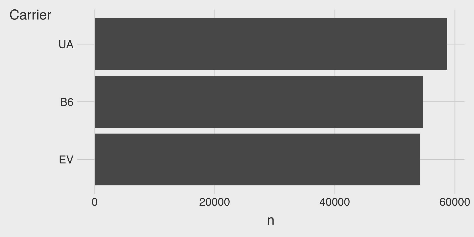
ggplot(data = top3_n,
       mapping = aes(x = __BLANK_1__,
                     y = __BLANK_2__)) +
  geom___BLANK_3__() +
  labs(y = "Carrier")   # label y-axis title
Show answer
ggplot(data = top3_n,
       mapping = aes(x = n,
                     y = fct_reorder(carrier, n))) +
  geom_col() +
  labs(y = "Carrier")
Question 9
🤖 Task: Create a data.frame named carrier_per_origin with the following variables:
origin: the origin airport
carrier: the airline carrier
n: the number of flights operated by each carrier from each origin airport
The carrier_per_origin data.frame should contain the count of flights for every carrier–origin combination.
carrier_per_origin <- flights |>
  __BLANK__ |>
  arrange(origin, -n)
Show answer
carrier_per_origin <- flights |>
  count(origin, carrier) |>
  arrange(origin, -n)
Discussion
Welcome to our Classwork 5 Discussion Board! 👋
This space is designed for you to engage with your classmates about the material covered in Classwork 5.
Whether you are looking to delve deeper into the content, share insights, or have questions about the content, this is the perfect place for you.
If you have any specific questions for Byeong-Hak (@bcdanl) regarding the Classwork 5 materials or need clarification on any points, don’t hesitate to ask here.
All comments will be stored here.
Let’s collaborate and learn from each other!