import pandas as pd
url_2024 = "https://bcdanl.github.io/data/esg_proj_2024_data.csv"
esg_proj_2024_data = pd.read_csv(url_2024)Beyond Profit: Analyzing ESG Risk and Stock Returns Across Sectors
DANL 210 Project
Project Submissions
Please submit the following three items for your project:
- A Python Script File (*.py) for Data Collection
Submit the scripts used to collect your data.
danl_210_LASTNAME_FIRSTNAME_stock_data_collection.py
- A CSV File (*.csv)
Export your final DataFrames as CSV files using the Python scripts above
danl_210_LASTNAME_FIRSTNAME_stock.csv
Contains daily stock market data from the beginning of 2024 to March 31, 2025, with the following columns:
Symbol: Company’s stock tickerName: Company nameDate: Trading dateOpen: Opening price on the dateHigh: Highest price on the dateLow: Lowest price on the dateClose: Closing price on the dateAdj Close: Adjusted close price accounting for splits and dividendsVolume: Trading volumeDividend: Cash dividend paid per share on the date (if any), as reported by Yahoo FinanceSplit: Stock split
Note: A CSV file must not exceed 30 MB.
- Jupyter Notebook File (*.ipynb) for Your Project Webpage
Filename: danl_210_LASTNAME_FIRSTNAME_stock_ESG.ipynb
Include your full Python code;(excluding the data collection scripts) and your project explanation, written clearly in text cells.
File size limit: 30 MB
Note: For data loading in Google Colab, you may use the file.upload() function.
- This lecture slide could be useful for data loading in Google Colab.
Deadline: Thursday, May 14, 11:59 P.M.
Project
- Collect the following data from Yahoo! Finance:
- Stock market data
- Conduct your data analysis using a Jupyter Notebook.
- Your analysis should center around the agenda: “Unifying ESG Metrics with Financial Analysis”
Project Data
- Below is the
esg_proj_2024_data,esg_proj_2025_data, andstock_history_2024DataFrames.
1. esg_proj_2024_data
- The
esg_proj_2024_dataDataFrame which provides a list of companies and associated information, including ESG scores as of March 31, 2024.
Variable Description
Symbol: a company’s ticker;Company Name: a company name;Sector: a sector a company belongs to;Industry: an industry a company belongs to;Country: a country a company belongs to;Market_Cap: a company’s market capitalization as of December 20, 2024 (Source: Nasdaq’s Stock Screener).- A company’s market capitalization is the value of the company that is traded on the stock market, calculated by multiplying the total number of shares by the present share price.
IPO_Year: the year a company first went public by offering its shares to be traded on a stock exchange.Total_ESG: The overall ESG (Environmental, Social, and Governance) risk score, summarizing the company’s exposure to ESG-related risks as of March 31, 2024. A lower score indicates lower risk.Environmental: The company’s exposure to environmental risks (e.g., emissions, energy use, environmental policy) as of March 31, 2024. A lower score indicates lower risk.Social: The company’s exposure to social risks (e.g., labor practices, human rights, diversity, and customer relations) as of March 31, 2024. A lower score indicates lower risk.Governance: The company’s exposure to governance-related risks (e.g., board structure, executive pay, shareholder rights, transparency) as of March 31, 2024. A lower score indicates lower risk.Controversy: A score reflecting the severity of recent ESG-related controversies involving the company as of March 31, 2024. Higher scores typically indicate greater or more serious controversies.
2. esg_proj_2025_data
- The
esg_proj_2025_dataDataFrame which provides a list of companies’ tickers and ESG scores as of March 31, 2025.
url_2025 = "https://bcdanl.github.io/data/esg_proj_2025_data.csv"
esg_proj_2024_data = pd.read_csv(url_2025)
3. stock_history_2024
- The
stock_history_2024DataFrame contains daily historical stock market data for the year 2024.
url = "https://bcdanl.github.io/data/stock_history_2024.csv"
stock_history_2024 = pd.read_csv(url)
Variable Description
Symbol: Company’s stock tickerDate: Trading dateYear: Trading yearOpen: Opening price on the dateHigh: Highest price on the dateLow: Lowest price on the dateClose: Close price adjusted for splitsAdj Close: Adjusted close price adjusted for splits and dividend and/or capital gain distributionsVolume: Trading volumeDividend: Cash dividend paid per share on the date (if any), as reported by Yahoo FinanceStock_Split: The ratio of any stock split that occurred on the given date.
Project Tasks
1. Collecting Historical Stock Data
For each company found in both the esg_proj_2024_data and esg_proj_2025_data DataFrames, employ the selenium library to retrieve:
- Daily stock prices from January 1, 2025, to April 1, 2026
- e.g., https://finance.yahoo.com/quote/MSFT/history/?p=MSFT&period1=1735689600&period2=1775001600
- 1735689600 = January 1, 2025
- 1775001600 = April 1, 2026
- e.g., https://finance.yahoo.com/quote/MSFT/history/?p=MSFT&period1=1735689600&period2=1775001600
- Requirements for Collecting Data from Yahoo! Finance:
- To locate the daily stock history table, use
WebDriverWait()withEC.presence_of_element_located()rather thanfind_element(). - Scrape at a moderate rate — use
time.sleep(random.uniform(5, y))between page visits to avoid overloading servers. - Handle potential errors gracefully using
try-exceptblocks. - Consider starting with the following setup for Selenium web scraping:
- To locate the daily stock history table, use
# %%
# =============================================================================
# Setup libraries
# =============================================================================
import time, random, os
import pandas as pd
import numpy as np
from selenium import webdriver
from selenium.webdriver.common.by import By
from selenium.webdriver.chrome.options import Options
from selenium.webdriver.support.ui import WebDriverWait
from selenium.webdriver.support import expected_conditions as EC
from selenium.common.exceptions import NoSuchElementException
from selenium.common.exceptions import TimeoutException
from selenium.common.exceptions import StaleElementReferenceException
from selenium.common.exceptions import WebDriverException

# %%
# =============================================================================
# Setup working directory
# =============================================================================
wd_path = 'PATHNAME_OF_YOUR_WORKING_DIRECTORY'
os.chdir(wd_path)


# %%
# =============================================================================
# Setup WebDriver with options
# =============================================================================
options = Options()
options.add_argument("window-size=1400,1200")  # Set window size
options.add_argument('--disable-blink-features=AutomationControlled')  # Prevent detection of automation by disabling blink features
options.page_load_strategy = 'eager'  # Load only essential content first, skipping non-critical resources

# Stability flags:
options.add_argument("--disable-dev-shm-usage")
options.add_argument("--no-sandbox")
options.add_argument("--disable-gpu")
options.add_argument("--disable-extensions")
options.add_argument("--disable-features=NetworkService")

driver = webdriver.Chrome(options=options)- Scraping web data falls into a legal gray area. In the U.S., scraping publicly available information is not illegal, but it is not always clearly allowed either.
- Most companies do not go after individuals for minor or non-commercial violations of their Terms of Service (ToS). Still, if the scraping causes harm, it can lead to legal trouble.
Dividend Cleaning
If you scrape historical data tables from each company’s page on Yahoo Finance (e.g., MSFT Historical Data), you can construct a DataFrame similar to the df_all DataFrame shown below.
The df_all DataFrame contains stock data for Apple Inc., Microsoft, and Nvidia from the beginning of 2024 through the end of Q1 2025:
import pandas as pd
df_all = pd.read_csv('https://bcdanl.github.io/data/aapl_msft_nvda_2024_2025.csv')
Note that some rows in the df_all DataFrame include dividend declarations rather than price and volume data (e.g., Apple Inc. on February 10, 2025). These dividend entries appear in the Open/High/Low/Close/Adj Close/Volume columns as strings like “0.25 Dividend”.
- Note: Apple Inc’s “0.25 Dividend” means that on that specific date, Apple Inc issued a cash dividend of $0.01 per share.
To separate these dividend entries from the actual stock trading data, we use the str.contains() method:
# Filter rows where the 'Open' column contains the word 'Dividend' (these represent dividend entries)
df_dividend = df_all[df_all['Open'].str.contains('Dividend', na=False)]

# Filter out dividend rows to keep only stock price data
df_stock = df_all[~df_all['Open'].str.contains('Dividend', na=False)]- At this point:
df_stockdoes not include dividend announcements.df_dividendincludes only dividend announcements.
We now clean and format the dividend information:
# Select only relevant columns for dividend data
df_dividend = df_dividend[['Date', 'Symbol', 'Open']]

# Copy 'Open' column (which contains dividend information) into a new column named 'Dividend'
df_dividend['Dividend'] = df_dividend['Open']

# Keep only the necessary columns: Date, Symbol, and Dividend
df_dividend = df_dividend[['Date', 'Symbol', 'Dividend']]

# Remove the text " Dividend" from the Dividend column to isolate the numeric value
df_dividend['Dividend'] = df_dividend['Dividend'].str.replace(' Dividend', '')

# Remove the text "s on any given ex-date include regular and any special dividends" from the Dividend column to isolate the numeric value
df_dividend['Dividend'] = df_dividend['Dividend'].str.replace('s on any given ex-date include regular and any special dividends', '')
Stock Split Cleaning
Some row in the df_dividend DataFrame from the “Dividend Cleaning” subsection includes stock splits rather than dividend data (e.g., Nvidia on June 10, 2024). These stock split entries appear in the Dividend column as strings like “10:1 Stock Splits”.
To separate these stock split entries from the actual stock trading data, again we use the str.contains() method:
# Filter rows where the 'Open' column contains the word 'Split' (these represent stock split entries)
df_split = df_dividend[df_dividend['Dividend'].str.contains('Split', na=False)]

# Filter out dividend rows to keep only dividend data
df_dividend = df_dividend[~df_dividend['Dividend'].str.contains('Split', na=False)]- At this point:
df_stockincludes only daily stock trading information.df_dividendincludes only dividend information.df_splitincludes only stock splits.
We now clean and format the split information:
# Select only relevant columns for dividend data
df_split = df_split[['Date', 'Symbol', 'Dividend']]

# Copy 'Open' column (which contains dividend information) into a new column named 'Split'
df_split['Split'] = df_split['Dividend']

# Keep only the necessary columns: Date, Symbol, and Split
df_split = df_split[['Date', 'Symbol', 'Split']]

# Remove the text " Stock Splits" from the Split column to isolate the numeric value
df_split['Split'] = df_split['Split'].str.replace(' Stock Splits', '')- Note: NVDA’s “10:1 Stock Split” means that each existing share was split into 10 shares.
- If you owned 1 share before June 10, 2024, you would own 10 shares after the split.
- To maintain consistency, Yahoo Finance retroactively adjusts all historical prices and volumes to reflect stock splits.
- For example, the table below shows NVDA’s adjusted stock prices and volumes from June 7–11, 2024:
Extracting the year and the month from a datetime variable
- To extract the year from a datetime variable in a pandas DataFrame, you can use the
.dt.yearaccessor. - To extract the month from a datetime variable in a pandas DataFrame, you can use the
.dt.monthaccessor.
# Sample DataFrame with string dates
data = {
    'Symbol': ['AAPL', 'MSFT', 'GOOG'],
    'Date': ['2024-12-29', '2024-12-30', '2025-01-03'],
    'Close': [130.21, 265.78, 122.34]
}

df = pd.DataFrame(data)

# Convert 'Date' column to datetime
df['Date'] = df['Date'].astype('datetime64[ns]')

# Extract year from 'Date' variable
df['Year'] = df['Date'].dt.year

# Extract month from 'Date' variable
df['Year'] = df['Date'].dt.month
2. Data Analysis
- If you are unable to complete the data collection tasks, use the
esg_proj_2024_dataandstock_history_2024DataFrames for your analysis. - If you successfully completed data collection, you may optionally incorporate
stock_history_2024as an additional source.
Below are the required components of your data analysis webpage.
Component 1 — Title
Provide a clear, concise title that reflects the focus of your project.
Component 2 — Introduction
- Background: Why are the research questions significant, relevant, or interesting?
- Statement of the Problem: What specific problem or question does this project address?
Component 3 — Data Collection
Describe how you retrieved historical stock data using selenium and pandas. Do not paste the collection code into the webpage — submit the .py script separately to Brightspace.
Component 4 — Descriptive Statistics
Provide summary statistics and distribution visualizations for both ESG and financial variables. Your descriptive statistics should include both ungrouped and sector/industry-grouped summaries.
Sector and Industry Group Analysis is a central focus of this project. When computing descriptive statistics, always group by Sector and/or Industry to reveal how ESG and financial characteristics differ across parts of the economy.
Questions to guide your grouped analysis:
- Which sectors have the highest and lowest average ESG risk scores?
- Which industries show the widest spread in stock returns or ESG scores?
- How does market capitalization vary by sector?
Component 5 — Exploratory Data Analysis
This is the core of your project. Structure your EDA around the three themes below. For each theme, state the questions you aim to answer, then address them with visualizations using seaborn (or lets-plot) and pandas.
🏭 Theme A: Sector and Industry Group Analysis
Compare ESG scores and financial performance across sectors and industries. This is the primary lens for your project. You may focus on sectors you find most interesting or analyze all of them.
📈 Theme B: ESG Time Trend (2024 → 2025)
Examine how ESG scores changed from 2024 to 2025, both overall and by sector.
📊 Theme C: Distribution of Stock Returns
Analyze the shape, spread, and group differences in the distribution of daily (or annual) stock returns.
What is a daily stock return?
A daily return measures the percentage change in a stock’s closing price from one trading day to the next:
\[ \text{Daily Return} = \frac{\text{Close}_t - \text{Close}_{t-1}}{\text{Close}_{t-1}} \times 100 \]
You can compute it in pandas using:
df = df.sort_values(['Symbol', 'Date'])
df['Daily_Return'] = df.groupby('Symbol')['Close'].pct_change() * 100
Suggested questions:
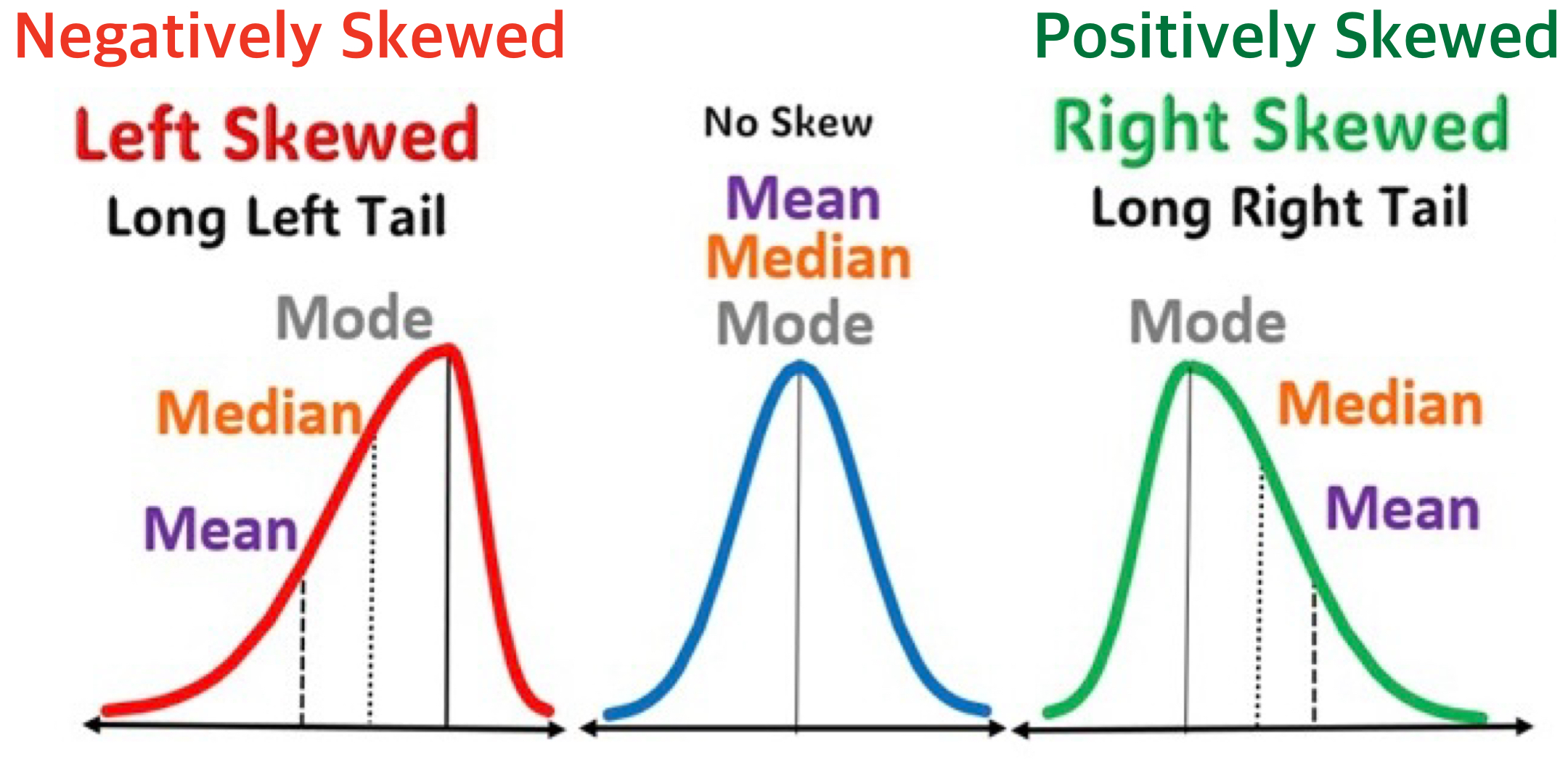
- What does the overall distribution of daily returns look like? Is it symmetric or skewed?
- Which sectors show the highest average returns? Which are the most volatile (wide spread)?
- Do high-ESG companies tend to have more stable returns than low-ESG companies?
- Are there companies with unusually large positive or negative returns (outliers)?
Suggested visualizations:
- Histograms plots of daily returns overall and by sector
- Box plots comparing return distributions across sectors or ESG tiers
- Scatter plots of average return vs. average ESG score, colored by sector
Component 6 — Significance of the Project
Discuss the real-world implications of your findings. What do your results suggest for investors, companies, or policymakers? How might ESG performance relate to financial outcomes?
Component 7 — References
- List all sources cited in the project, including web addresses for online references.
- Note if any part of the code or write-up was guided by generative AI (e.g., ChatGPT). There is no penalty for this.
- Note if any part of the work resulted from collaboration with classmates. There is no penalty for collaboration, as long as shared portions are clearly identified.
Interpreting ESG Data 🧾
ESG data helps investors evaluate a company’s sustainability profile and exposure to long-term environmental, social, and governance risks. Here’s how to interpret each metric:
🔢 Total ESG Risk Score
- What it means: A composite score reflecting the company’s overall exposure to ESG-related risks.
- How to interpret:
- Lower score = lower risk → Better ESG performance.
- Higher score = higher risk → More vulnerable to ESG-related issues.
- Example: A company with total_ESG = 15 is considered to have lower ESG risk than one with total_ESG = 30.
- Lower score = lower risk → Better ESG performance.
🌍 Environmental Risk Score
- What it measures: Exposure to environmental risks such as:
- Carbon emissions
- Energy efficiency
- Waste management
- Climate change strategy
- Carbon emissions
- Interpretation:
- Lower score → better environmental practices.
- Higher score → more environmental liabilities or poor sustainability measures.
🏛 Governance Risk Score
- What it measures: Exposure to governance-related risks, such as:
- Board structure and independence
- Executive compensation
- Shareholder rights
- Transparency and ethics
- Board structure and independence
- Interpretation:
- Lower score suggests better corporate oversight.
- Higher score suggests poor governance structures.
🚨 Controversy Level
- What it measures: Reflects recent ESG-related controversies involving the company.
- Scale: Usually ranges from 0 (no controversies) to 5 (severe and ongoing issues).
- Interpretation:
- Low score (0–1): Minimal or no controversies.
- High score (4–5): Major controversies — potential reputational or legal risks.
- Note: A company may have good ESG scores but still be flagged due to a high controversy score.
🧠 ESG Score Summary
| Metric | Good Score | Bad Score |
|---|---|---|
| total_ESG | Low | High |
| Environmental | Low | High |
| Social | Low | High |
| Governance | Low | High |
| Controversy | 0–1 | 4–5 |
General Tips on Data Visualization 📈
Distribution
When describing the distribution of a variable, we are typically interested in several key characteristics:
- Center: The central tendency of the data, such as the mean or median, which indicates the typical or average value.
- Spread: How spread the values are within the variable, showing the range and standard deviation of values.
- Common Values: Identifying frequent values and the mode.
- Rare Values: Recognizing unusual or infrequent values.
- Shape: The overall shape of the distribution, such as whether it’s symmetric, skewed left or right, or having multiple groups with multiple peaks.
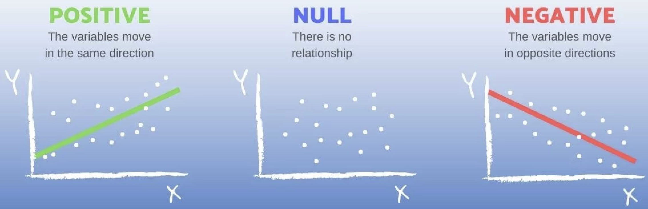
Relationship Between Two Variables
- Start with determining whether the two variables have a positive association, a negative association, or no association.
- E.g., A negative slope in the fitted line indicates that sales decrease as the price increases, while a positive slope would indicate that sales increase with price. A zero slope means that there is no relationship between sales and price; changes in price do not affect sales.
- Input on the x-axis; output on the y-axis
- By convention, the input (or predictor) variable is plotted on the x-axis, and the output (or response) variable on the y-axis.
- This helps visualize potential relationships—though it shows correlation, not necessarily causation.
- Correlation does not necessarily mean causation.
- When a question asks you to describe how the relationship varies by another categorical variable, examine both the direction of the slope (negative, positive, or none) from the fitted line and the steepness of the slope (steep or shallow).
- The slope of the fitted straight line is the rate at which the “y” variable (like grades) changes as the “x” variable (like study hours) changes. In simple terms, it shows how much one thing goes up or down when the other thing changes.
- For example, a comment such as, “The plot shows a negative relationship between sales and price” does not address how the relationship differs by brand.
- The focus is on the relationship, not the distribution.
- While adding a comment on the distribution of a single variable can be helpful, the question is primarily about the relationship between the two variables.
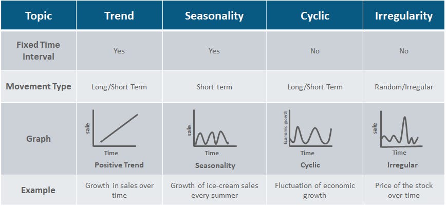
Time Trend of a Variable
Here are some general tips for describing the time trend of a variable:
- Identify the Overall Trend — Is the variable moving upward, downward, or staying roughly constant over time?
- Note Patterns and Cycles — Look for repeating seasonal fluctuations (monthly or quarterly) or longer-term cycles that suggest persistent influences.
- Highlight Significant Fluctuations — Describe any sharp increases, decreases, or irregular spikes and connect them to real-world events if possible.
Describing ESG time trends (2024 → 2025) specifically:
- Does the average ESG risk score across all companies go up or down? A lower score in 2025 would indicate improving sustainability practices industry-wide.
- Which sectors improved most? Which got worse? A diverging bar chart of year-over-year ESG score changes by sector is especially effective here.
- Do the Environmental, Social, and Governance sub-scores move together, or do they diverge? For example, some sectors may improve on environmental metrics while social scores worsen.
- Is the ESG trend correlated with stock price trends over the same period? Companies with improving ESG scores may also show stronger price performance.
Interpreting Visualization
- Be specific.
- Avoid vague statements. Below examples do not actually explain what the patterns are.
- “The plot shows how the time trend of a stock price varies across sectors, with each sector having a unique best fitting line and scatter pattern”
- “The trend shows the evolution of stock price in the market over time”
- Clearly describe what is the pattern—and how it differs across categories.
- Avoid vague statements. Below examples do not actually explain what the patterns are.
- Add Narration:
- Connect the visualization to real-world phenomena and/or your idea that could help explain it, adding insight into what is happening.
How to Extract Year from a Datetime Variable in pandas
If you would like to extract the year from a datetime variable in a pandas DataFrame, you can use the .dt.year accessor. Below is an example:
import pandas as pd

# Sample DataFrame with string dates
data = {
    'Symbol': ['AAPL', 'MSFT', 'GOOG'],
    'Date': ['2024-12-29', '2024-12-30', '2025-01-03'],
    'Close': [130.21, 265.78, 122.34]
}

df = pd.DataFrame(data)

# Convert 'Date' column to datetime
df['Date'] = pd.to_datetime(df['Date'])

# Extract year from 'Date' column
df['Year'] = df['Date'].dt.year
This will add a new Year variable to the df DataFrame containing the corresponding year for each date.
Uploading CSV Files to Google Colab via Google Drive
When you work in Google Colab, your notebook runs on a temporary cloud computer.
To access files you already have in your Google Drive (like a CSV), you first need to mount your Drive.
from google.colab import drive
drive.mount('/content/drive')
What this code does
from google.colab import drive
Imports Colab’s built-in tool for connecting to Google Drive.drive.mount("/content/drive")
Connects (mounts) your Google Drive into Colab at the folder path:
/content/drive
What you will see after running it
- Colab will ask you to sign in to your Google account.
- You will approve permission for Colab to access your Drive.
- After that, your Drive files will appear under:
/content/drive/MyDrive/
Example: read a CSV file from Google Drive
import pandas as pd

df = pd.read_csv("/content/drive/MyDrive/path/to/your_file.csv")
Rubric
Project Write-up
| Attribute | Very Deficient (1) | Somewhat Deficient (2) | Acceptable (3) | Very Good (4) | Outstanding (5) |
|---|---|---|---|---|---|
| 1. Quality of research questions | • Not stated or very unclear • Entirely derivative • Anticipate no contribution |
• Stated somewhat confusingly • Slightly interesting, but largely derivative • Anticipate minor contributions |
• Stated explicitly • Somewhat interesting and creative • Anticipate limited contributions |
• Stated explicitly and clearly • Clearly interesting and creative • Anticipate at least one good contribution |
• Articulated very clearly • Highly interesting and creative • Anticipate several important contributions |
| 2. Quality of data visualization | • Very poorly visualized • Unclear • Unable to interpret figures |
• Somewhat visualized • Somewhat unclear • Difficulty interpreting figures |
• Mostly well visualized • Mostly clear • Acceptably interpretable |
• Well organized • Well thought-out visualization • Almost all figures clearly interpretable |
• Very well visualized • Outstanding visualization • All figures clearly interpretable |
| 3. Quality of exploratory data analysis | • Little or no critical thinking • Little or no understanding of data analytics concepts with Python |
• Rudimentary critical thinking • Somewhat shaky understanding of data analytics concepts with Python |
• Average critical thinking • Understanding of data analytics concepts with Python |
• Mature critical thinking • Clear understanding of data analytics concepts with Python |
• Sophisticated critical thinking • Superior understanding of data analytics concepts with Python |
| 4. Quality of business/economic analysis | • Little or no critical thinking • Little or no understanding of business/economic concepts |
• Rudimentary critical thinking • Somewhat shaky understanding of business/economic concepts |
• Average critical thinking • Understanding of business/economic concepts |
• Mature critical thinking • Clear understanding of business/economic concepts |
• Sophisticated critical thinking • Superior understanding of business/economic concepts |
| 5. Quality of writing | • Very poorly organized • Very difficult to read • Many typos and grammatical errors |
• Somewhat disorganized • Somewhat difficult to read • Numerous typos and grammatical errors |
• Mostly well organized • Mostly easy to read • Some typos and grammatical errors |
• Well organized • Easy to read • Very few typos or grammatical errors |
• Very well organized • Very easy to read • No typos or grammatical errors |
| 6. Quality of Jupyter Notebook usage | • Very poorly organized • Many redundant warning/error messages • Inappropriate code to produce outputs |
• Somewhat disorganized • Numerous warning/error messages • Misses important code |
• Mostly well organized • Some warning/error messages • Provides appropriate code |
• Well organized • Very few warning/error messages • Provides advanced code |
• Very well organized • No warning/error messages • Proposes highly advanced code |
Data Collection
| Evaluation | Description | Criteria |
|---|---|---|
| 1 (Very Deficient) | - Very poorly implemented - Data is unreliable. |
- Poor web scraping practices with selenium, leading to unreliable or incorrect data from Yahoo Finance.- Inadequate use of pandas, resulting in poorly structured DataFrames. |
| 2 (Somewhat Deficient) | - Somewhat effective implementation - Data has minor reliability issues. |
- Basic web scraping with selenium that sometimes fails to capture all relevant data accurately.- Basic use of pandas, but with occasional issues in data structuring. |
| 3 (Acceptable) | - Effective web scraping with selenium, capturing most required data from Yahoo Finance.- Adequate use of pandas to structure data in a mostly logical format. |
|
| 4 (Very Good) | - Well-implemented and organized - Data is reliable. |
- Thorough web scraping with selenium that consistently captures accurate and complete data from Yahoo Finance.- Skillful use of pandas for clear and logical data structuring. |
| 5 (Outstanding) | - Exceptionally implemented - Data is highly reliable. |
- Expert web scraping with selenium, capturing detailed and accurate data from Yahoo Finance without fail.- Expert use of pandas to create exceptionally well-organized DataFrames that facilitate easy analysis. |
👥 Social Risk Score