import pandas as pd
import numpy as npHomework 5
Data Transfomration with pandas II
📌 Directions
- Submit your Jupyter Notebook (*.ipynb) to Brightspace using this format:
danl-210-hw5-LASTNAME-FIRSTNAME.ipynb
(e.g.,danl-210-hw5-choe-byeonghak.ipynb)
- Due: April 27, 2026, 11:59 P.M.
- Questions? Email Prof. Choe: bchoe@geneseo.edu
For this Section, use the above Python libraries and the following four DataFrames from Global Gourmet Selections, which represent the company’s operations:
customers– Contains customer-related information, including unique customer IDs, names, and contact details.orders– Provides an overview of order details, including relevant transaction information.order_details– Records individual order line items by linking each product to a specific order.products– Stores product-related details, such as product IDs, names, and pricing.
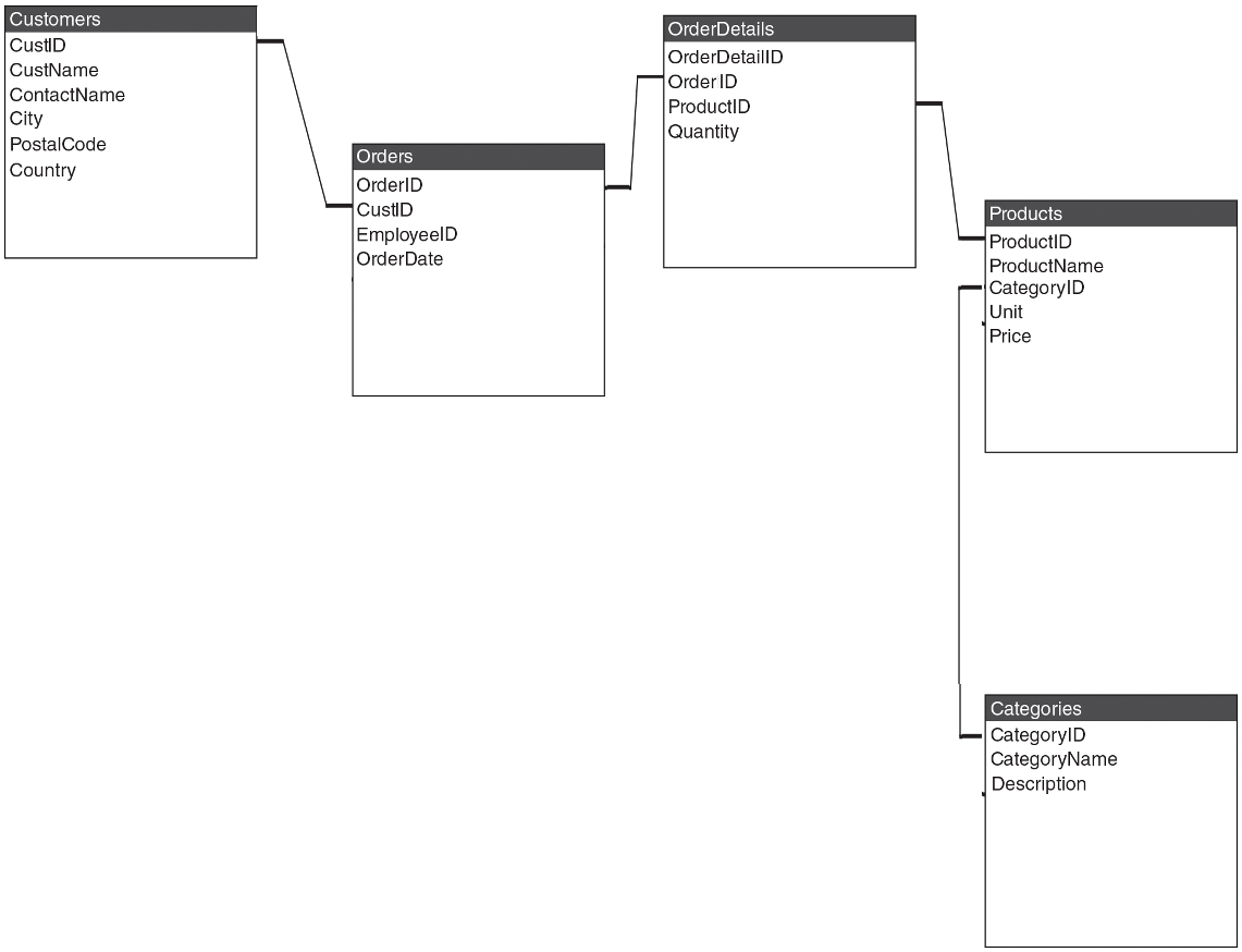
Additionally, the categories DataFrame offers metadata on product categories, including unique identifiers, names, and descriptions.
DataFrames
categories = pd.read_csv('https://bcdanl.github.io/data/gourmet-Categories.csv')
customers = pd.read_csv('https://bcdanl.github.io/data/gourmet-Customers2.csv')
orders = pd.read_csv('https://bcdanl.github.io/data/gourmet-Orders2.csv')
order_details = pd.read_csv('https://bcdanl.github.io/data/gourmet-OrderDetails2.csv')
products = pd.read_csv('https://bcdanl.github.io/data/gourmet-Products2.csv')
0. categories DataFrame (containing 8 observations)
| CategoryID | CategoryName | Description |
|---|---|---|
| 1 | Beverages | Soft drinks coffees teas beers and ales |
| 2 | Condiments | Sweet and savory sauces relishes spreads and seasonings |
| 3 | Confections | Desserts candies and sweet breads |
| 4 | Dairy Products | Cheeses |
| 5 | Grains/Cereals | Breads crackers pasta and cereal |
| 6 | Meat/Poultry | Prepared meats |
| 7 | Produce | Dried fruit and bean curd |
| 8 | Seafood | Seaweed and fish |
CategoryID(int64): Unique identifier for each product category in thecategoriesDataFrame.CategoryName(object): The name of the category.Description(object): A textual description providing details about the category.
1. customers DataFrame with its first 15 observations
| CustID | CustName | ContactName | City | PostalCode | Country |
|---|---|---|---|---|---|
| 1 | Alfreds Futterkiste | Maria Anders | Berlin | 12209 | Germany |
| 2 | Ana Trujillo Emparedados y helados | Ana Trujillo | Mexico D.F. | NA | Mexico |
| 3 | Antonio Moreno Taqueria | Antonio Moreno | Mexico D.F. | NA | Mexico |
| 4 | Around the Horn | Thomas Hardy | London | WA1 1DP | UK |
| 5 | Berglunds snabbkop | Christina Berglund | Lulea | S-958 22 | Sweden |
| 6 | Blauer See Delikatessen | Hanna Moos | Mannheim | 68306 | Germany |
| 7 | Blondel pere et fils | Frederique Citeaux | Strasbourg | 67000 | France |
| 8 | Bolido Comidas preparadas | Martin Sommer | Madrid | 28023 | Spain |
| 9 | Bon app’ | Laurence Lebihans | Marseille | 13008 | France |
| 10 | Bottom-Dollar Marketse | Elizabeth Lincoln | Tsawassen | T2F 8M4 | Canada |
| 11 | B’s Beverages | Victoria Ashworth | London | EC2 5NT | UK |
| 12 | Cactus Comidas para llevar | Patricio Simpson | Buenos Aires | 1010 | Argentina |
| 13 | Centro comercial Moctezuma | Francisco Chang | Mexico D.F. | 5022 | Mexico |
| 14 | Chop-suey Chinese | Yang Wang | Bern | 3012 | Switzerland |
| 15 | Comercio Mineiro | Pedro Afonso | Sao Paulo | 05432-043 | Brazil |
CustID(int64): Unique identifier for each customer in thecustomersDataFrame.CustName(object): The name of the customer’s company.ContactName(object): The name of the primary contact person at the company.City(object): The city where the customer is located.PostalCode(object): The postal or ZIP code of the customer’s address.Country(object): The country of the customer.
2. orders DataFrame with its first 15 observations
| OrderID | CustID | EmployeeID | OrderDate |
|---|---|---|---|
| 10248 | 90 | 5 | 7/4/96 |
| 10249 | 81 | 6 | 7/5/96 |
| 10250 | 34 | 4 | 7/8/96 |
| 10251 | 84 | 3 | 7/8/96 |
| 10252 | 76 | 4 | 7/9/96 |
| 10253 | 34 | 3 | 7/10/96 |
| 10254 | 14 | 5 | 7/11/96 |
| 10255 | 68 | 9 | 7/12/96 |
| 10256 | 88 | 3 | 7/15/96 |
| 10257 | 35 | 4 | 7/16/96 |
| 10258 | 20 | 1 | 7/17/96 |
| 10259 | 13 | 4 | 7/18/96 |
| 10260 | 55 | 4 | 7/19/96 |
| 10261 | 61 | 4 | 7/19/96 |
| 10262 | 65 | 8 | 7/22/96 |
OrderID(int64): Unique identifier for each order in theordersDataFrame.CustID(int64): Identifier linking to the customer who placed the order in thecustomersDataFrame.EmployeeID(int64): Identifier for the employee handling the order.OrderDate(object): The date when the order was placed.
3. order_details DataFrame with its first 15 observations
| OrderDetail_ID | OrderID | ProductID | Quantity |
|---|---|---|---|
| 1 | 10248 | 11 | 12 |
| 2 | 10248 | 42 | 10 |
| 3 | 10248 | 72 | 5 |
| 4 | 10249 | 14 | 9 |
| 5 | 10249 | 51 | 40 |
| 6 | 10250 | 41 | 10 |
| 7 | 10250 | 51 | 35 |
| 8 | 10250 | 65 | 15 |
| 9 | 10251 | 22 | 6 |
| 10 | 10251 | 57 | 15 |
| 11 | 10251 | 65 | 20 |
| 12 | 10252 | 20 | 40 |
| 13 | 10252 | 33 | 25 |
| 14 | 10252 | 60 | 40 |
| 15 | 10253 | 31 | 20 |
OrderDetail_ID(int64): Unique identifier for each record in theorder_detailsDataFrame.OrderID(int64): Identifier linking each record to a specific order in theordersDataFrame.ProductID(int64): Identifier linking the record to a product in theproductsDataFrame.Quantity(int64): The number of units ordered.
4. products DataFrame with its first 15 observations
| ProductID | ProductName | CategoryID | Unit | Price |
|---|---|---|---|---|
| 1 | Chais | 1 | 10 boxes x 20 bags | 18.00 |
| 2 | Chang | 1 | 24 - 12 oz bottles | 19.00 |
| 3 | Aniseed Syrup | 2 | 12 - 550 ml bottles | 10.00 |
| 4 | Chef Anton’s Cajun Seasoning | 2 | 48 - 6 oz jars | 22.00 |
| 5 | Chef Anton’s Gumbo Mix | 2 | 36 boxes | 21.35 |
| 6 | Grandma’s Boysenberry Spread | 2 | 12 - 8 oz jars | 25.00 |
| 7 | Uncle Bob’s Organic Dried Pears | 7 | 12 - 1 lb pkgs. | 30.00 |
| 8 | Northwoods Cranberry Sauce | 2 | 12 - 12 oz jars | 40.00 |
| 9 | Mishi Kobe Niku | 6 | 18 - 500 g pkgs. | 97.00 |
| 10 | Ikura | 8 | 12 - 200 ml jars | 31.00 |
| 11 | Queso Cabrales | 4 | 1 kg pkg. | 21.00 |
| 12 | Queso Manchego La Pastora | 4 | 10 - 500 g pkgs. | 38.00 |
| 13 | Konbu | 8 | 2 kg box | 6.00 |
| 14 | Tofu | 7 | 40 - 100 g pkgs. | 23.25 |
| 15 | Genen Shouyu | 2 | 24 - 250 ml bottles | 15.50 |
ProductID(int64): Unique identifier for each product in theproductsDataFrame.ProductName(object): The name of the product.CategoryID(int64): Identifier linking the product to a category in thecategoriesDataFrame.Unit(object): The packaging or standard unit in which the product is soldPrice(float): The cost of a single unit of the product (in USD)
Question 1
- Write a three-line code snippet to display the following summaries of the
ordersDataFrame:
<class 'pandas.core.frame.DataFrame'>
RangeIndex: 196 entries, 0 to 195
Data columns (total 4 columns):
 #   Column      Non-Null Count  Dtype
---  ------      --------------  -----
 0   OrderID     196 non-null    int64
 1   CustID      196 non-null    int64
 2   EmployeeID  196 non-null    int64
 3   OrderDate   196 non-null    object
dtypes: int64(3), object(1)
memory usage: 6.2+ KB
<class 'pandas.core.frame.DataFrame'>
RangeIndex: 196 entries, 0 to 195
Data columns (total 4 columns):
# Column Non-Null Count Dtype
--- ------ -------------- -----
0 OrderID 196 non-null int64
1 CustID 196 non-null int64
2 EmployeeID 196 non-null int64
3 OrderDate 196 non-null datetime64[ns]
dtypes: datetime64[ns](1), int64(3)
memory usage: 6.2 KB
Show answer
orders.info()
orders['OrderDate'] = orders['OrderDate'].astype('datetime64[ns]')
orders.info()
Question 2
Write a code snippet to produce the following output of descriptive statistics:
       ProductName       Price
count           77   77.000000
unique          77         NaN
top          Chais         NaN
freq             1         NaN
mean           NaN   28.866364
std            NaN   33.815111
min            NaN    2.500000
25%            NaN   13.250000
50%            NaN   19.500000
75%            NaN   33.250000
max            NaN  263.500000
Show answer
products[['ProductName', 'Price']].describe(include="all")Question 3
Fill in the blank to count the number of observations from the customers DataFrame where the customer’s Country is not USA.
customers[_______________________________________________].shape[0]
Show answer
customers[customers['Country'] != 'USA'].shape[0]Question 4
Fill in the blank to count the number of observations from the customers DataFrame where the customer’s ContactName starts with B or P.
customers[_______________________________________________]
Show answer
customers[customers['ContactName'].between('B', 'C') | customers['ContactName'].between('P', 'Q') ]Question 5
Write a code snippet to identify the country or countries with the highest number of missing values in the PostalCode variable of the customers DataFrame.
Show answer
(
  customers[customers['PostalCode'].isna()]['Country']
  .value_counts()
  .reset_index()
  .nlargest(1, 'count', keep = 'all')
)
Question 6
Write a code snippet using the order_details DataFrame to count the number of unique products ordered.
The total number of distinct products ordered is 77.
Show answer
order_details['ProductID'].nunique()Question 7
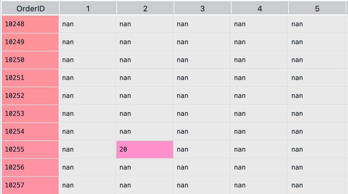
Write a code snippet to reshape the order_details DataFrame so that each OrderID is a row and each ProductID becomes a column with values equal to the corresponding Quantity.
     OrderID   1     2   3   4   5   6   7  ...  70  71   72  73    74  75  76  77
0      10248 NaN   NaN NaN NaN NaN NaN NaN  ... NaN NaN  5.0 NaN   NaN NaN NaN NaN
1      10249 NaN   NaN NaN NaN NaN NaN NaN  ... NaN NaN  NaN NaN   NaN NaN NaN NaN
2      10250 NaN   NaN NaN NaN NaN NaN NaN  ... NaN NaN  NaN NaN   NaN NaN NaN NaN
3      10251 NaN   NaN NaN NaN NaN NaN NaN  ... NaN NaN  NaN NaN   NaN NaN NaN NaN
4      10252 NaN   NaN NaN NaN NaN NaN NaN  ... NaN NaN  NaN NaN   NaN NaN NaN NaN
..       ...  ..   ...  ..  ..  ..  ..  ..  ...  ..  ..  ...  ..   ...  ..  ..  ..
191    10439 NaN   NaN NaN NaN NaN NaN NaN  ... NaN NaN  NaN NaN  30.0 NaN NaN NaN
192    10440 NaN  45.0 NaN NaN NaN NaN NaN  ... NaN NaN  NaN NaN   NaN NaN NaN NaN
193    10441 NaN   NaN NaN NaN NaN NaN NaN  ... NaN NaN  NaN NaN   NaN NaN NaN NaN
194    10442 NaN   NaN NaN NaN NaN NaN NaN  ... NaN NaN  NaN NaN   NaN NaN NaN NaN
195    10443 NaN   NaN NaN NaN NaN NaN NaN  ... NaN NaN  NaN NaN   NaN NaN NaN NaN

[196 rows x 78 columns]- The following displays the first 10 rows and the first 6 columns of the resulting DataFrame:
Show answer
(
  order_details
  .pivot(index='OrderID',
         columns='ProductID',
         values='Quantity')
  .reset_index()
)
Question 8
Write a code snippet to display the following new DataFrame showing each category along with the number of unique products in the products DataFrame.
| CategoryName | count |
|---|---|
| Confections | 13 |
| Beverages | 12 |
| Condiments | 12 |
| Seafood | 12 |
| Dairy Products | 10 |
| Grains/Cereals | 7 |
| Meat/Poultry | 6 |
| Produce | 5 |
Show answer
(
  products
  .merge(categories, on="CategoryID", how="left")[['CategoryName']]
  .value_counts()
  .reset_index()
)
Question 9
Write a code snippet to create the following new DataFrame, ProductID_11, showing the Quantity ordered for ProductID 11. Then, write a one-line Pandas code to compute the total quantity of this product ordered using the ProductID_11 DataFrame.
| OrderDetail_ID | OrderID | ProductID | ProductName | Quantity |
|---|---|---|---|---|
| 1 | 10248 | 11 | Queso Cabrales | 12 |
| 130 | 10296 | 11 | Queso Cabrales | 12 |
| 211 | 10327 | 11 | Queso Cabrales | 50 |
| 281 | 10353 | 11 | Queso Cabrales | 12 |
| 314 | 10365 | 11 | Queso Cabrales | 24 |
| 426 | 10407 | 11 | Queso Cabrales | 30 |
| 492 | 10434 | 11 | Queso Cabrales | 6 |
| 514 | 10442 | 11 | Queso Cabrales | 30 |
| 517 | 10443 | 11 | Queso Cabrales | 6 |
The total quantity ordered for ProductID 11 is 182.Note that 182 is calculated as follows: \[ 182 = 12 + 12 + 50 + 12 + 24 + 30 + 6 + 30 + 6 \]
Show answer
ProductID_11 = (
    order_details
    .merge(products,
           on="ProductID",
           how="left")
    .query('ProductID == 11')
    [['OrderDetail_ID', 'OrderID', 'ProductID', 'ProductName', 'Quantity']]
)

ProductID_11['Quantity'].sum()
Question 10
- Write a code snippet to determine how many unique CustomerID-EmployeeID pairs exist in the
ordersDataFrame. Then, count how many times each EmployeeID appears in these unique pairs and return the resulting DataFrame as below:
| EmployeeID | count |
|---|---|
| 1 | 23 |
| 2 | 18 |
| 3 | 26 |
| 4 | 31 |
| 5 | 10 |
| 6 | 17 |
| 7 | 14 |
| 8 | 25 |
| 9 | 6 |
- What does this
countvariable above tell us?
Show answer
(
  orders[['EmployeeID', 'CustID']]
  .value_counts()
  .reset_index()[['EmployeeID']]
  .value_counts()
  .reset_index()
)
count variable tells us the number of customers whose orders are handled by each employee.
Question 11
- Write a code snippet to compute the total order cost for customers in Mexico, expressed in Mexican Pesos (MXN).
- Begin by adding a new variable, PriceMXN, to the
productsDataFrame, which converts the Price to pesos by multiplying it by 20.604.
- Begin by adding a new variable, PriceMXN, to the
Total cost of orders made by customers in Mexico: 120771.58 MXN
Show answer
products['PriceMXN'] = products['Price'] * 20.604

q17 = (
  order_details
  .merge(products, on="ProductID", how="left")
  .merge(orders, on="OrderID", how="left")
  .merge(customers, on="CustID", how="left")
  .query('Country == "Mexico"')
)

q17['Cost'] = q17['PriceMXN'] * q17['Quantity']
q17['Cost'].sum()