beer_markets <- read_csv('https://bcdanl.github.io/data/beer_markets_all.csv')Classwork 12
Data Transformation
Part 1 - Beer Markets
Question 1
Use skimr::skim() to get summary statistics (e.g, mean, standard deviation, median, minimum, maximum) about the price for one bottle of beer (12 oz) for each brand when there was promo and when there was not.
Answer:
Code
q1 <- beer_markets |>
mutate(bottle_floz = 12 * beer_floz) |>
group_by(brand) |>
skim()Question 2
- For each household, calculate the number of beer transactions.
- For each household, calculate the proportion of each beer brand choice.
Answer:
Code
q2 <- beer_markets %>%
count(hh, brand) %>%
group_by(hh) %>%
mutate(n_tot = sum(n)) %>% # n_tot : the number of beer transactions
arrange(hh, brand) %>%
mutate( prop = n / n_tot ) # prop: the proportion of each beer brand choiceQuestion 3
Among households that purchased BUD LIGHT at least once, what proportion only bought BUD LIGHT?
Among households that purchased BUSCH LIGHT at least once, what proportion only bought BUSCH LIGHT?
Among households that purchased COORS LIGHT at least once, what proportion only bought COORS LIGHT?
Among households that purchased MILLER LITE at least once, what proportion only bought MILLER LITE?
Among households that purchased NATURAL LIGHT at least once, what proportion only bought NATURAL LIGHT?
Which beer brand does have the largest proportion of such loyal consumers?
Answer:
Code
q3 <- beer_markets %>%
mutate(bud = ifelse(brand=="BUD LIGHT", 1, 0), # 1 if brand=="BUD LIGHT"; 0 otherwise
busch = ifelse(brand=="BUSCH LIGHT", 1, 0),
coors = ifelse(brand=="COORS LIGHT", 1, 0),
miller = ifelse(brand=="MILLER LITE", 1, 0),
natural = ifelse(brand=="NATURAL LIGHT", 1, 0),
.after = hh) %>%
select(hh:natural) %>% # select the variables we need
group_by(hh) %>%
summarise(n_transactions = n(), # number of beer transactions for each hh
n_bud = sum(bud), # number of BUD LIGHT transactions for each hh
n_busch = sum(busch),
n_coors = sum(coors),
n_miller = sum(miller),
n_natural = sum(natural)
) %>%
summarise(loyal_bud = sum(n_transactions == n_bud) / sum(n_bud > 0),
# sum(n_transactions == n_bud) : the number of households that purchased BUD LIGHT only
# sum(n_bud > 0) : the number of households that purchased BUD LIGHT at least once.
loyal_busch = sum(n_transactions == n_busch) / sum(n_busch > 0),
loyal_coors = sum(n_transactions == n_coors) / sum(n_coors > 0),
loyal_miller = sum(n_transactions == n_miller) / sum(n_miller > 0),
loyal_natural = sum(n_transactions == n_natural) / sum(n_natural > 0)
)Part 2 - NYC Housing Markets
nyc_housing_sales <- read_csv('https://bcdanl.github.io/data/nyc_housing_sales_2006-2023.csv')Question 4
Use skimr::skim() to get summary statistics (e.g, mean, standard deviation, median, minimum, maximum) about sale_price for each borough.
Answer:
Code
q4 <- nyc_housing_sales |>
group_by(borough) |>
skim(sale_price)| Name | group_by(nyc_housing_sale… |
| Number of rows | 200913 |
| Number of columns | 22 |
| _______________________ | |
| Column type frequency: | |
| numeric | 1 |
| ________________________ | |
| Group variables | borough |
Variable type: numeric
| skim_variable | borough | n_missing | complete_rate | mean | sd | p0 | p25 | p50 | p75 | p100 | hist |
|---|---|---|---|---|---|---|---|---|---|---|---|
| sale_price | Bronx | 0 | 1 | 470269.4 | 403341.4 | 1 | 315000 | 417000 | 545000 | 17062000 | ▇▁▁▁▁ |
| sale_price | Brooklyn | 0 | 1 | 828342.5 | 899816.4 | 1 | 417000 | 620000 | 920000 | 25500000 | ▇▁▁▁▁ |
| sale_price | Manhattan | 0 | 1 | 8076326.2 | 7885675.7 | 1 | 3076642 | 6000000 | 10600000 | 77100000 | ▇▁▁▁▁ |
| sale_price | Queens | 0 | 1 | 611494.2 | 1046660.6 | 1 | 375000 | 540000 | 750000 | 139874900 | ▇▁▁▁▁ |
| sale_price | Staten Island | 0 | 1 | 494624.0 | 389728.7 | 1 | 350000 | 455000 | 595000 | 35000000 | ▇▁▁▁▁ |
Question 5
Add the new variable, age, to data.frame, nyc_housing_sales, using the year and year_built variables.
Answer:
Code
nyc_housing_sales <- nyc_housing_sales |>
mutate(age = year - year_built,
.before = year)Question 6
Provide both (1) ggplot code and (2) a simple comment to describe how the daily trend of the distribution of sale_price varies by borough, on average.
Answer:
Code
ggplot(nyc_housing_sales,
aes(x = sale_date, y = sale_price)) +
geom_point(size = .25, alpha = .1) +
geom_smooth(aes(color = borough, fill = borough)) +
facet_wrap(borough~., scales = 'free_y')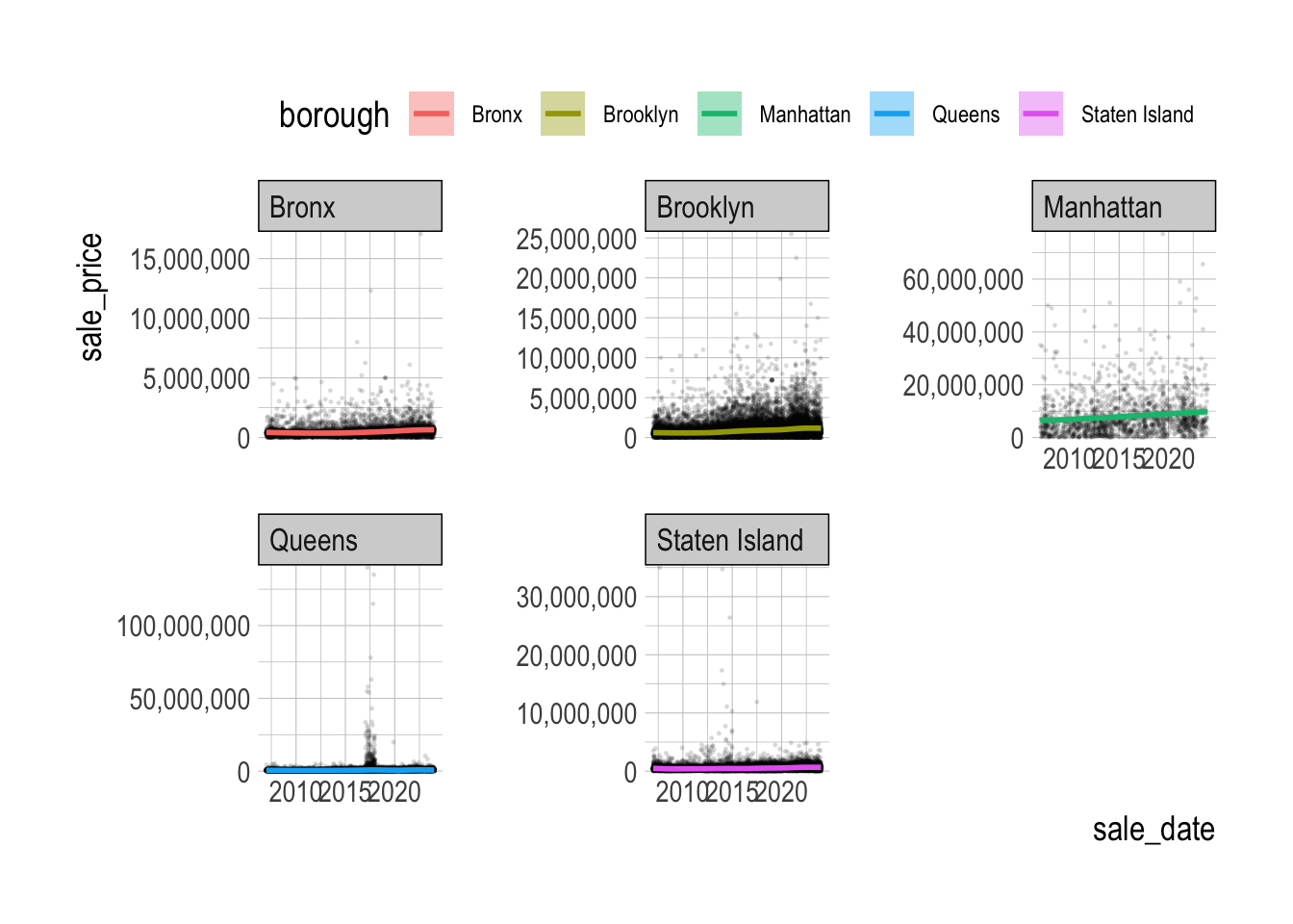
- Removing outliers for each borough could lead to a better visualization:
Code
q6 <- nyc_housing_sales |>
group_by(borough, year) |>
mutate(lower = quantile(sale_price, .1), # 10th percentile
upper = quantile(sale_price, .9) # 90th percentile
) |>
filter(sale_price < upper, sale_price > lower) # non-outliers
ggplot(q6,
aes(x = sale_date, y = log10(sale_price))) +
geom_point(size = .25, alpha = .1) +
geom_smooth(aes(color = borough, fill = borough)) +
facet_wrap(borough~.)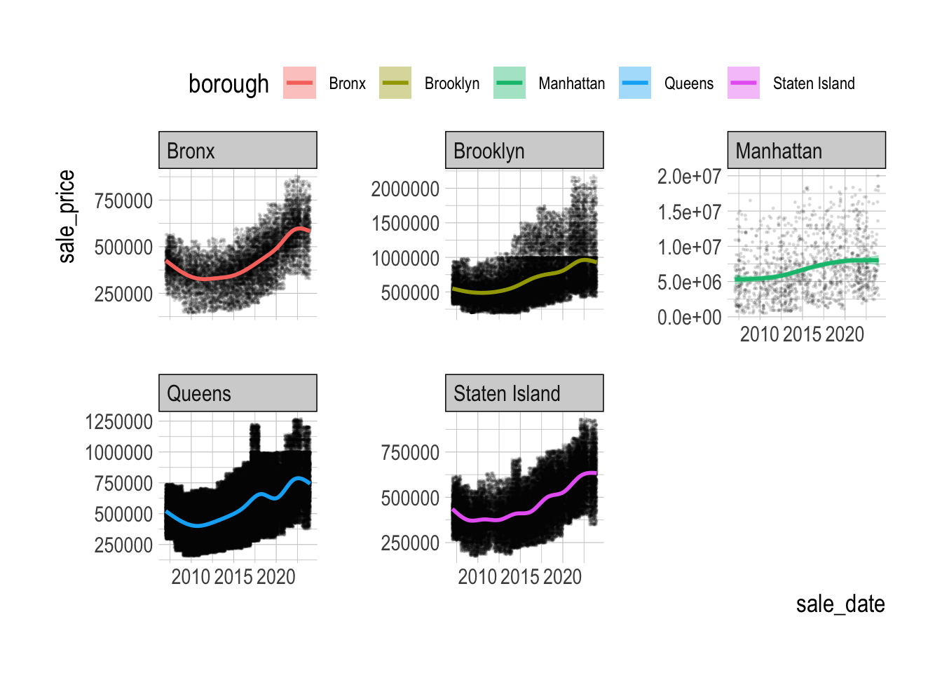
Question 7
Identify the neighborhood with the highest average housing sales price for each month of each year.
Answer:
Code
q7 <- nyc_housing_sales |>
mutate(borough_neighborhood = str_c(borough, ', ', neighborhood)) |> # to display borough info
group_by(year, month, borough_neighborhood) |>
summarise(mean_sale_price = mean(sale_price, na.rm = T),
n = n()) |>
slice_max(mean_sale_price, n = 1)