library(tidyverse)
library(skimr)Fall 2023 DANL 200-04/05 Final Exams
Load R packages
- Here we are loading all the R packages we need for the Final Exam, so that you do not need to load the R packages in your code.
Question 1
- Below is the data.frame for Question 1.
uk_soccer <- read_csv("https://bcdanl.github.io/data/premier_league_2022.csv")- Below is the data.frame,
uk_soccer.
Code
rmarkdown::paged_table(uk_soccer,
                       options = list(rows.print = 20,
                                      cols.print = 5,
                                      pages.print = 0,
                                      paged.print = F
)) nrow(uk_soccer)[1] 380ncol(uk_soccer)[1] 10table(uk_soccer$Quarter)< table of extent 0 >table(uk_soccer$Quarter_Num)< table of extent 0 >Variable description
Date: The date when the match was played
HomeTeam: The home team
AwayTeam: The away team
FTHG: The home team’s goals after the match ends (full-time)
FTAG: The away team’s goals after the match ends (full-time)
FTR: The match result after the match ends (full-time)
- The value of FTR is “H” if FTHG is greater than FTAG;
- The value of FTR is “D” if FTHG is equal to FTAG;
- The value of FTR is “A” if FTHG is less than FTAG.
HTHG: The home team’s goals at the half-time of the match
HTAG: The away team’s goals at the half-time of the match
HTR: The match result at the halftime of the match
- The value of HTR is “H” if HTHG is greater than HTAG;
- The value of HTR is “D” if HTHG is equal to HTAG;
- The value of HTR is “A” if HTHG is less than HTAG.
nrow(uk_soccer)[1] 380ncol(uk_soccer)[1] 10table(uk_soccer$HomeTeam)
       Arsenal    Aston Villa      Brentford       Brighton        Burnley
            19             19             19             19             19
       Chelsea Crystal Palace        Everton          Leeds      Leicester
            19             19             19             19             19
     Liverpool       Man City     Man United      Newcastle        Norwich
            19             19             19             19             19
   Southampton      Tottenham        Watford       West Ham         Wolves
19 19 19 19 19 table(uk_soccer$AwayTeam)
       Arsenal    Aston Villa      Brentford       Brighton        Burnley
            19             19             19             19             19
       Chelsea Crystal Palace        Everton          Leeds      Leicester
            19             19             19             19             19
     Liverpool       Man City     Man United      Newcastle        Norwich
            19             19             19             19             19
   Southampton      Tottenham        Watford       West Ham         Wolves
19 19 19 19 19 table(uk_soccer$FTR)
  A   D   H
129 88 163 table(uk_soccer$HTR)
  A   D   H
101 151 128 class(uk_soccer$Date)[1] "character"class(uk_soccer$HomeTeam)[1] "character"class(uk_soccer$AwayTeam)[1] "character"class(uk_soccer$FTHG)[1] "numeric"class(uk_soccer$FTAG)[1] "numeric"class(uk_soccer$HTHG)[1] "numeric"class(uk_soccer$HTAG)[1] "numeric"Q1a.
Create the following two data.frames, tott_home and tott_away:
- tott_home includes all the observations whose HomeTeam is “Tottenham”.
- tott_home includes only the two variables, FTR and HTR.
- tott_away includes all the observations whose AwayTeam is “Tottenham”.
- tott_away includes only the two variables, FTR and HTR.
Answer:
Code
tott_home <- uk_soccer |>
  filter(HomeTeam == "Tottenham") |>
  select(FTR, HTR)

tott_away <- uk_soccer |>
  filter(AwayTeam == "Tottenham") |>
select(FTR, HTR)- Below is the data.frame,
tott_home.
Code
rmarkdown::paged_table(tott_home,
                       options = list(rows.print = 20,
                                      cols.print = 5,
                                      pages.print = 0,
                                      paged.print = F
)) - Below is the data.frame,
tott_away.
Code
rmarkdown::paged_table(tott_away,
                       options = list(rows.print = 20,
                                      cols.print = 5,
                                      pages.print = 0,
                                      paged.print = F
                                      ))
Q1b.
- Create the following four data.frames.
- home_htr that counts the number of observations for each value of HTR in tott_home.
- home_ftr that counts the number of observations for each value of FTR in tott_home.
- away_htr that counts the number of observations for each value of HTR in tott_away.
- away_ftr that counts the number of observations for each value of FTR in tott_away.
Answer:
Code
home_htr <- tott_home |> count(HTR)
home_ftr <- tott_home |> count(FTR)
away_htr <- tott_away |> count(HTR)
away_ftr <- tott_away |> count(FTR)- Below is the data.frame,
home_htr.
Code
rmarkdown::paged_table(home_htr,
                       options = list(rows.print = 20,
                                      cols.print = 5,
                                      pages.print = 0,
                                      paged.print = F
)) - Below is the data.frame,
home_ftr.
Code
rmarkdown::paged_table(home_ftr,
                       options = list(rows.print = 20,
                                      cols.print = 5,
                                      pages.print = 0,
                                      paged.print = F
)) - Below is the data.frame,
away_htr.
Code
rmarkdown::paged_table(away_htr,
                       options = list(rows.print = 20,
                                      cols.print = 5,
                                      pages.print = 0,
                                      paged.print = F
)) - Below is the data.frame,
away_ftr.
Code
rmarkdown::paged_table(away_ftr,
                       options = list(rows.print = 20,
                                      cols.print = 5,
                                      pages.print = 0,
                                      paged.print = F
                                      ))
Q1c. [Out of Coverage in Spring 2024, DANL 200-02]
- Create the following two data.frames:
- home_results is created using home_ftr and home_htr;
- away_results is created using away_ftr and away_htr.
Answer:
Code
home_results <-
  left_join(home_ftr, home_htr,
            by = c('FTR' = 'HTR')) |>
  rename(result = FTR,
         FTR = n.x, HTR = n.y) |>
  mutate(tott_location = "Home", .before = 1)

away_results <-
  left_join(away_ftr, away_htr,
            by = c('FTR' = 'HTR')) |>
  rename(result = FTR, FTR = n.x, HTR = n.y) |>
mutate(tott_location = "Away", .before = 1)- Below is the data.frame, home_results.
Code
rmarkdown::paged_table(home_results,
                       options = list(rows.print = 20,
                                      cols.print = 5,
                                      pages.print = 0,
                                      paged.print = F
)) - Variable result in home_results is:
- A if the away team won the match;
- D if the home and away teams made draws;
- H if the home team won the match.
- Variable FTR in home_results is variable n in home_ftr;
- Variable HTR in home_results is variable n in home_htr;
- Below is the data.frame, away_results.
Code
rmarkdown::paged_table(away_results,
                       options = list(rows.print = 20,
                                      cols.print = 5,
                                      pages.print = 0,
                                      paged.print = F
)) - Variable result in away_results is:
- A if the away team won the match;
- D if the home and away teams made draws;
- H if the home team won the match.
- Variable FTR in away_results is variable n in away_ftr;
- Variable HTR in away_results is variable n in away_htr;
Q1d.
- For variable result in home_results data.frame, replace:
- “A” with “Lose”;
- “D” with “Draw”;
- “H” with “Win”.
- For variable result in away_results data.frame, replace:
- “A” with “Win”;
- “D” with “Draw”;
- “H” with “Lose”.
Answer:
Code
home_results <- home_results |>
  mutate(result = ifelse(result == "A", "Lose",
                         ifelse(result == "D", "Draw", "Win")))
away_results <- away_results |>
  mutate(result = ifelse(result == "A", "Win",
ifelse(result == "D", "Draw", "Lose")))- Below is the data.frame, home_results.
Code
rmarkdown::paged_table(home_results,
                       options = list(rows.print = 20,
                                      cols.print = 5,
                                      pages.print = 0,
                                      paged.print = F
)) - Below is the data.frame, away_results.
Code
rmarkdown::paged_table(away_results,
                       options = list(rows.print = 20,
                                      cols.print = 5,
                                      pages.print = 0,
                                      paged.print = F
                                      ))
Q1e. [Out of Coverage in Spring 2024, DANL 200-02]
- Create the data.frame, tott_results, that combines the two data.frames home_results and away_results.
Answer:
Code
home_results <- home_results |>
  pivot_longer(cols = FTR:HTR,
               names_to = "time",
               values_to = "count")

away_results <- away_results |>
  pivot_longer(cols = FTR:HTR,
               names_to = "time",
               values_to = "count")

tott_results <- home_results |>
rbind(away_results)- Below is the data.frame, tott_results.
Code
rmarkdown::paged_table(tott_results,
                       options = list(rows.print = 40,
                                      cols.print = 5,
                                      pages.print = 0,
                                      paged.print = F
                                      ))
Q1f.
- Provide R code to recreate the ggplot figure illustrating how Tottenham Hotspur’s result varies by time and tott_location.
- Variable time is “Half-Time” if it is “HTR” in Q1e.
- Variable time is “Full-Time” if it is “FTR” in Q1e.
- Ensure that the order of values in result, time, and tott_location are properly set to recreate the ggplot.
Answer:
Code
df <- tott_results |>
  mutate(result = factor(result,
                         levels = c("Win", "Draw", "Lose")),
         time = ifelse(time == "FTR",
                       "Full-Time", "Half-Time"),
         time = factor(time,
                       levels = c("Half-Time", "Full-Time")),
         tott_location = factor(tott_location,
                                levels = c("Home", "Away")))

ggplot(df, aes(x = result,
             y = count, fill = time)) +
  geom_col(position = 'dodge') +
  facet_wrap(.~tott_location) +
  scale_fill_wsj()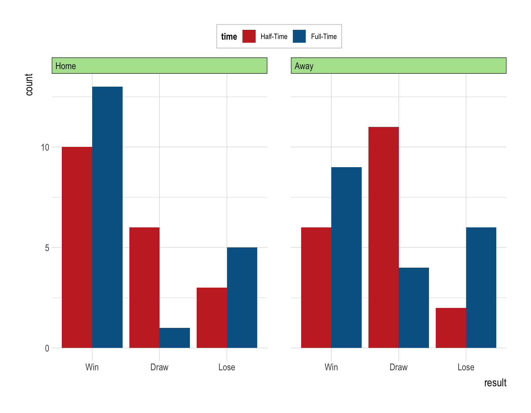
Q1g.
- Provide a comment to illustrate how Tottenham Hotspur’s performance varies by time and tott_location using the visualization in Q1f.
Answer:
Question 2
- The following describes the context of the data.frame,
organ_donations.- In the United States, people are not signed up to be organ donors by default. In most states, you are assumed to not be an organ donor. When you sign up for a driver’s license, you can choose to opt in to the organ donation program.
- It is probably not surprising that organ donation rates in the US are considerably lower than in other countries where organ donation is opt-out - you are assumed to be a donor unless you actively choose not to be.
- Outside of the opt-in and opt-out varieties of organ donation, there’s also “active choice.” Under active choice, when you sign up for a driver’s license, you are asked to choose whether or not to be a donor. You can choose yes or no, but now the “no” option is actively checking the “no” box rather than skipping the question entirely as you can with opt-in approaches.
- Some policymakers have been advocating for active choice, with a goal of increasing donation rates, and 41 US states were using an “active choice” frame for an organ donor registration question at their Department of Motor Vehicles (DMV) in 2014.
- So does active choice work? In July 2011, the state of California switched from opt-in to active choice.
- Below is the data.frame for Question 1.
organ_donations <- read_csv('https://bcdanl.github.io/data/organ_donations.csv')- Below is the data.frame,
organ_donations.
Code
rmarkdown::paged_table(organ_donations,
                       options = list(rows.print = 20,
                                      cols.print = 5,
                                      pages.print = 0,
                                      paged.print = F
)) nrow(organ_donations)[1] 162ncol(organ_donations)[1] 4table(organ_donations$Quarter)
Q12011 Q12012 Q22011 Q32011 Q42010 Q42011
27 27 27 27 27 27 table(organ_donations$Quarter_Num)
 1  2  3  4  5  6
27 27 27 27 27 27
Variable description
State: The stateQuarter: Quarter of observation, in “Q”QYYYY formatRate: Organ donation rateQuarter_Num: Quarter of observation in numerical format.1 = Quarter 4, 2010
Q2a
- Add the new variable,
Cali, to the data.frame,organ_donations.CaliisTRUEifState == 'California'.CaliisFALSEotherwise.
- Locate the
Calivariable after theStatevariable in the data.frame.
Answer:
Code
organ_donations <- organ_donations |>
  mutate(Cali = State == 'California',
.after = State)- Below is the data.frame,
organ_donations.
Code
rmarkdown::paged_table(organ_donations,
                       options = list(rows.print = 20,
                                      cols.print = 5,
                                      pages.print = 0,
                                      paged.print = F
)) - Answer:
Q2b. [Out of Coverage in Spring 2024, DANL 200-02]
-Separate the variable Quarter into quarter and year.
quarterisQ2,Q2,Q3, orQ4.yearis2010,2011, or2012.
Answer:
Code
organ_donations <- organ_donations |>
separate(Quarter, into = c('quarter', 'year'), sep = 2)- Answer:
Q2c. [Out of Coverage in Spring 2024, DANL 200-02]
- Count the number of unique values of
States.- In other words, how many states are in the data.frame,
organ_donations?
- In other words, how many states are in the data.frame,
- Then, create the data.frame
CA_tmp, which has only the California’s observations fromorgan_donations.
Answer:
Code
n_st <- nrow(organ_donations |> group_by(State) |> count())

CA_tmp <- organ_donations |>
filter(Cali == T)- Below is the data.frame,
CA_tmp.
Code
rmarkdown::paged_table(CA_tmp,
                       options = list(rows.print = 20,
                                      cols.print = 5,
                                      pages.print = 0,
                                      paged.print = F
)) - Answer:
Q2d. [Out of Coverage in Spring 2024, DANL 200-02]
Create the data.frame,
CA, which repeats stacking the data.frame,CA_tmp, so that the number of observations inCAis the same as the one inorgan_donations.- Note: Use
rbind().
- Note: Use
Then, change the name of variable,
Rate, withca_ratein the data.frameCA.Then, keep only the
ca_ratevariable from theCAdata.frame.
Answer:
Code
CA <- rbind(CA_tmp, CA_tmp, CA_tmp, CA_tmp, CA_tmp,
            CA_tmp, CA_tmp, CA_tmp, CA_tmp, CA_tmp,
            CA_tmp, CA_tmp, CA_tmp, CA_tmp, CA_tmp,
            CA_tmp, CA_tmp, CA_tmp, CA_tmp, CA_tmp,
            CA_tmp, CA_tmp, CA_tmp, CA_tmp, CA_tmp,
            CA_tmp, CA_tmp) |>
  rename(ca_rate = Rate) |>
select(ca_rate)- Below is the data.frame,
CA.
Code
rmarkdown::paged_table(CA,
                       options = list(rows.print = 20,
                                      cols.print = 5,
                                      pages.print = 0,
                                      paged.print = F
)) - Answer:
Q2e. [Out of Coverage in Spring 2024, DANL 200-02]
- Use the data.frame
CAto add the new variable,diff_rate, to the data.frame,organ_donationsdiff_rateis (ca_rateinCA) - (Rateinorgan_donations).- Note:
cbind()can be useful.
Answer:
Code
organ_donations <- cbind(organ_donations, CA) |>
  mutate(diff_rate = ca_rate - Rate,
.after = Rate)- Below is the data.frame,
organ_donations.
Code
rmarkdown::paged_table(organ_donations,
                       options = list(rows.print = 20,
                                      cols.print = 5,
                                      pages.print = 0,
                                      paged.print = F
)) - Answer:
Q2f.
Consider the resulting data.frame in Q2e.
For each
Quarter_Num, calculate the mean value ofdiff_rate.
Answer:
Code
Q2f <- organ_donations |>
  group_by(Quarter_Num) |>
summarise(mean_diff = mean(diff_rate, na.rm = T))- Below is the resulting data.frame.
Code
rmarkdown::paged_table(Q2f,
                       options = list(rows.print = 20,
                                      cols.print = 5,
                                      pages.print = 0,
                                      paged.print = F
)) - Answer:
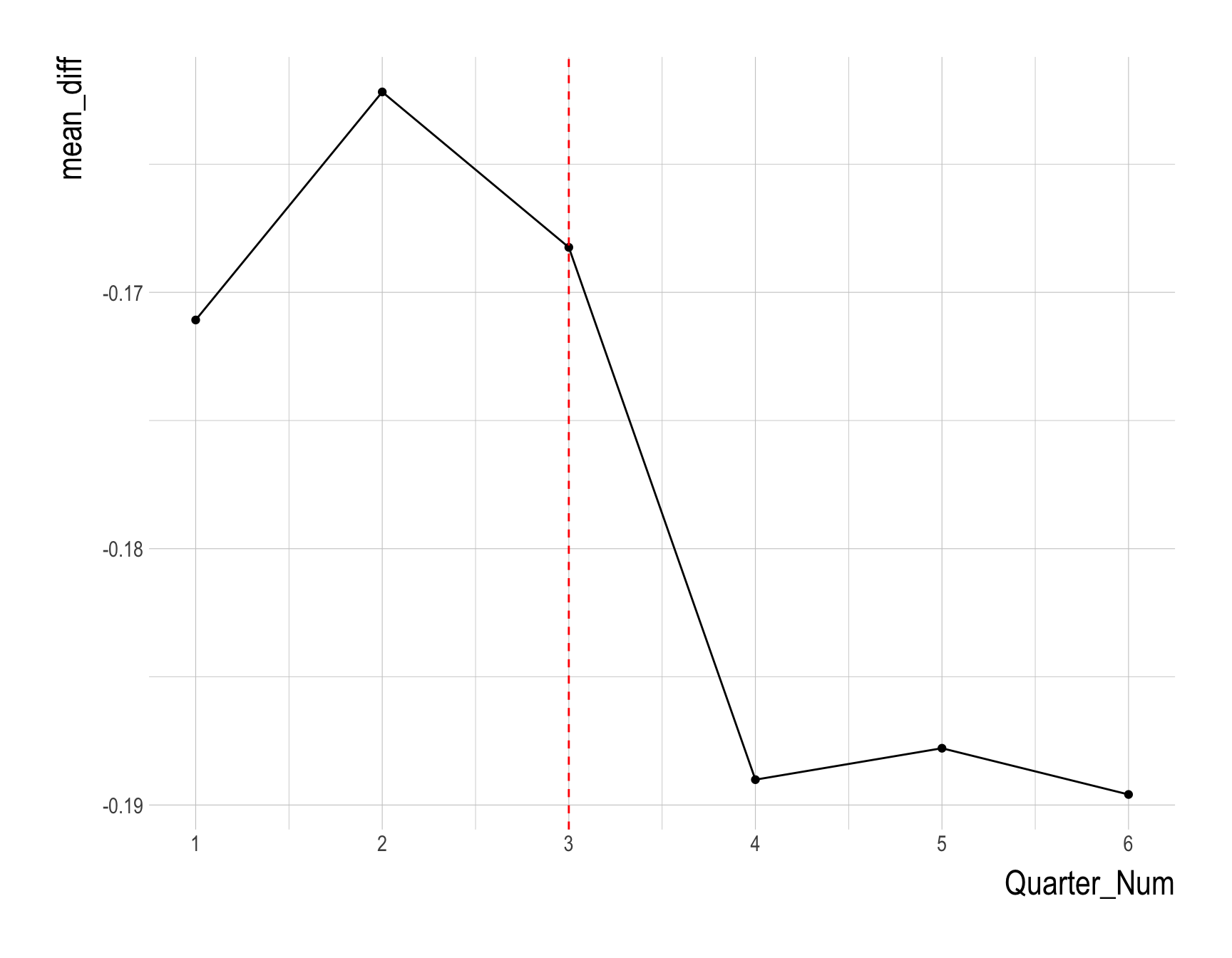
Q2g.
- Provide a ggplot code to visualize the quarterly trend of
mean_diffusing the resulting data.frame of Q2f, as follows.
Answer:
Code
ggplot(Q2f, aes(Quarter_Num, mean_diff)) +
  geom_line() +
  geom_point() +
  geom_vline(xintercept = 3, color = 'red', lty = 2) +
  scale_x_continuous(breaks = 1:6) +
  theme(axis.title.x = element_text(size = rel(2)),
        axis.title.y = element_text(size = rel(2))
        )
- Answer:
Q2h.
- Using the resulting visualization in Q2g, discuss the following question:
- What is the effect of active choice frame on organ donation rate?
Answer:
- Answer:
Question 3
- Below is the data.frame for Question 3.
taylor_albums <- read_csv("https://bcdanl.github.io/data/taylor_albums.csv")- Below is the data.frame,
taylor_albums.
Code
rmarkdown::paged_table(taylor_albums |>
                         relocate(metacritic_score, user_score,
                                  .after = album_name),
                       options = list(rows.print = 20,
                                      cols.print = 5,
                                      pages.print = 0,
                                      paged.print = F
)) nrow(taylor_albums)[1] 16ncol(taylor_albums)[1] 5unique(taylor_albums$album_name) [1] "Taylor Swift" "The Taylor Swift Holiday Collection"
[3] "Beautiful Eyes" "Fearless"
[5] "Speak Now" "Red"
[7] "1989" "reputation"
[9] "Lover" "folklore"
[11] "evermore" "Fearless (Taylor's Version)"
[13] "Red (Taylor's Version)" "Midnights"
[15] "Speak Now (Taylor's Version)" "1989 (Taylor's Version)" Variable description
album_name: The name of the album. NA if the song was released separately from one of Taylor’s studio albums or EPs.
metacritic_score: The official album rating from metacritic.
user_score: The user rating from metacritic.
ep: Logical. Is the album a full studio album (FALSE) or an extended play (TRUE).
album_release: The date the album was released, in the format (YYYY-MM-DD).
Q3a.
- Provide R code to recreate the ggplot figure illustrating the Taylor Swift’s Album’s metacritic_scores
Answer:
Code
ggplot(data = taylor_albums |> filter(!is.na(metacritic_score)),
       aes(x = metacritic_score,
           y = fct_reorder(album_name, metacritic_score))) +
  geom_col(aes(fill = album_name), show.legend = FALSE) +
  scale_fill_albums() +
  labs(y = NULL)  # labs() is not necessary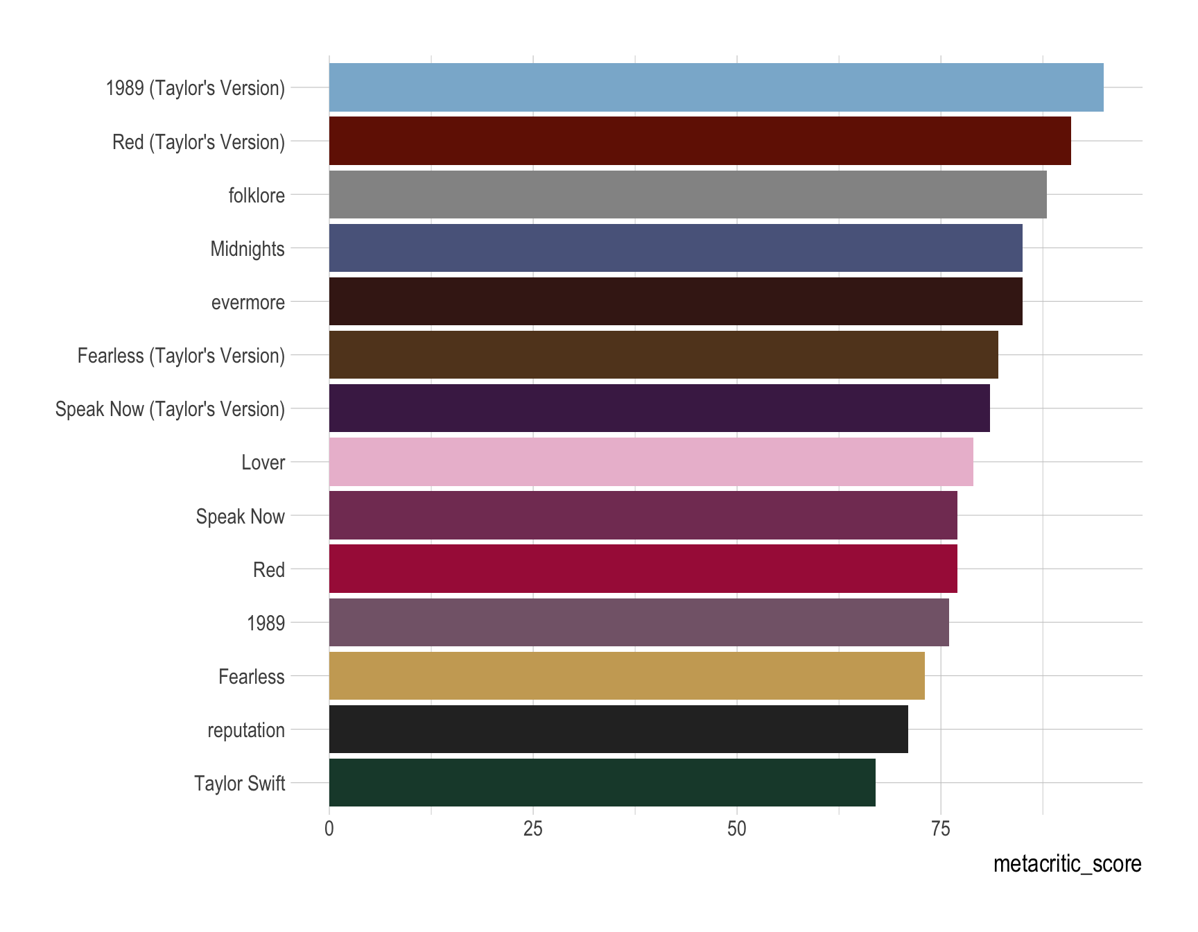
Question 4.
The following is the description and the data.frame for Question 4:
The Nobel Prize in Economic Science in 2021 goes to David Card, Joshua Angrist and Guido Imbens, for their empirical contributions to labor economics, and for their methodological contributions to the analysis of causal relationships.
They have provided us with new insights about the labor market and shown what conclusions about cause and effect can be drawn from natural experiments. Their approach has spread to other fields and revolutionized empirical research.
The following data.frame comes from the 1980 US Census and covers men born 1930–1939, which is used by Joshua Angrist and Alan Krueger’s research article.
- Below is the data.frame for Question 1.
ak91_age <- read_csv(
  'https://bcdanl.github.io/data/ak91_age.csv'
)- Below is the data.frame,
ak91_age.
Code
rmarkdown::paged_table(ak91_age |>
                         mutate(logW = round(logW, 2),
                                Educ = round(Educ, 2),
                                ),
                       options = list(rows.print = 40,
                                      cols.print = 6,
                                      pages.print = 0,
                                      paged.print = F
)) nrow(ak91_age)[1] 40ncol(ak91_age)[1] 6Variable description
- QoB: Quarter of birth
- YoB: Year of birth (1930, 1931, …, 1939)
- YoBQ: Year and quarter of birth (1930 Q1, 1930 Q2, …, 1939 Q4)
- logW: the natural log of weekly wage
- Educ: Years of education
- Q4:
TRUEif QoB == 4;FALSEotherwise.
Q4a.
Provide a ggplot code to recreate the following figure.
Answer:
Code
ggplot(ak91_age, aes(x = YoBQ, y = Educ)) +
  geom_line() +
geom_point( aes(color = Q4), size = 2.25 ) 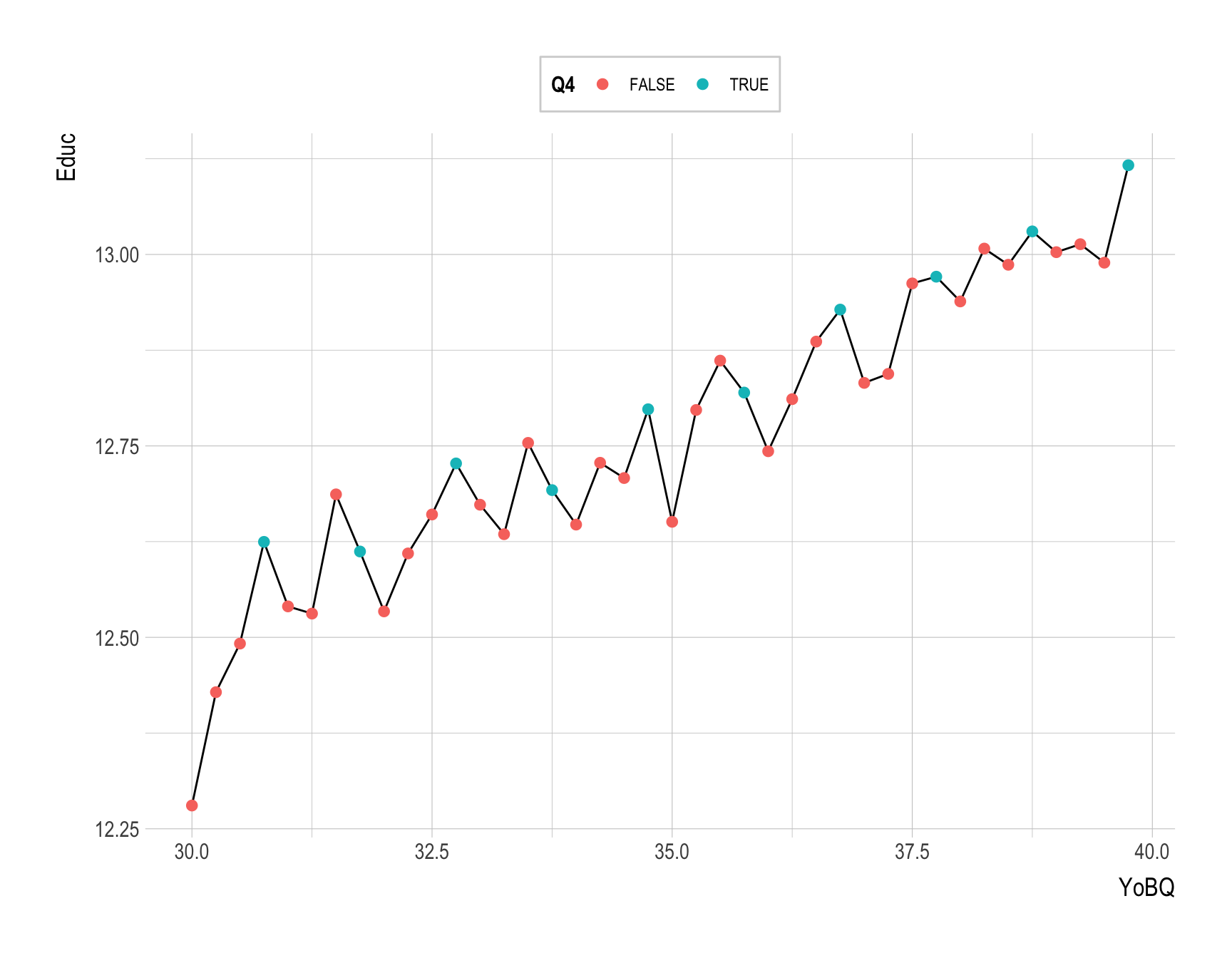
Q4b.
Provide a ggplot code to recreate the following figure.
Answer:
Code
ggplot(ak91_age, aes(x = YoBQ, y = logW)) +
  geom_line() +
geom_point( aes(color = Q4), size = 2.25 ) 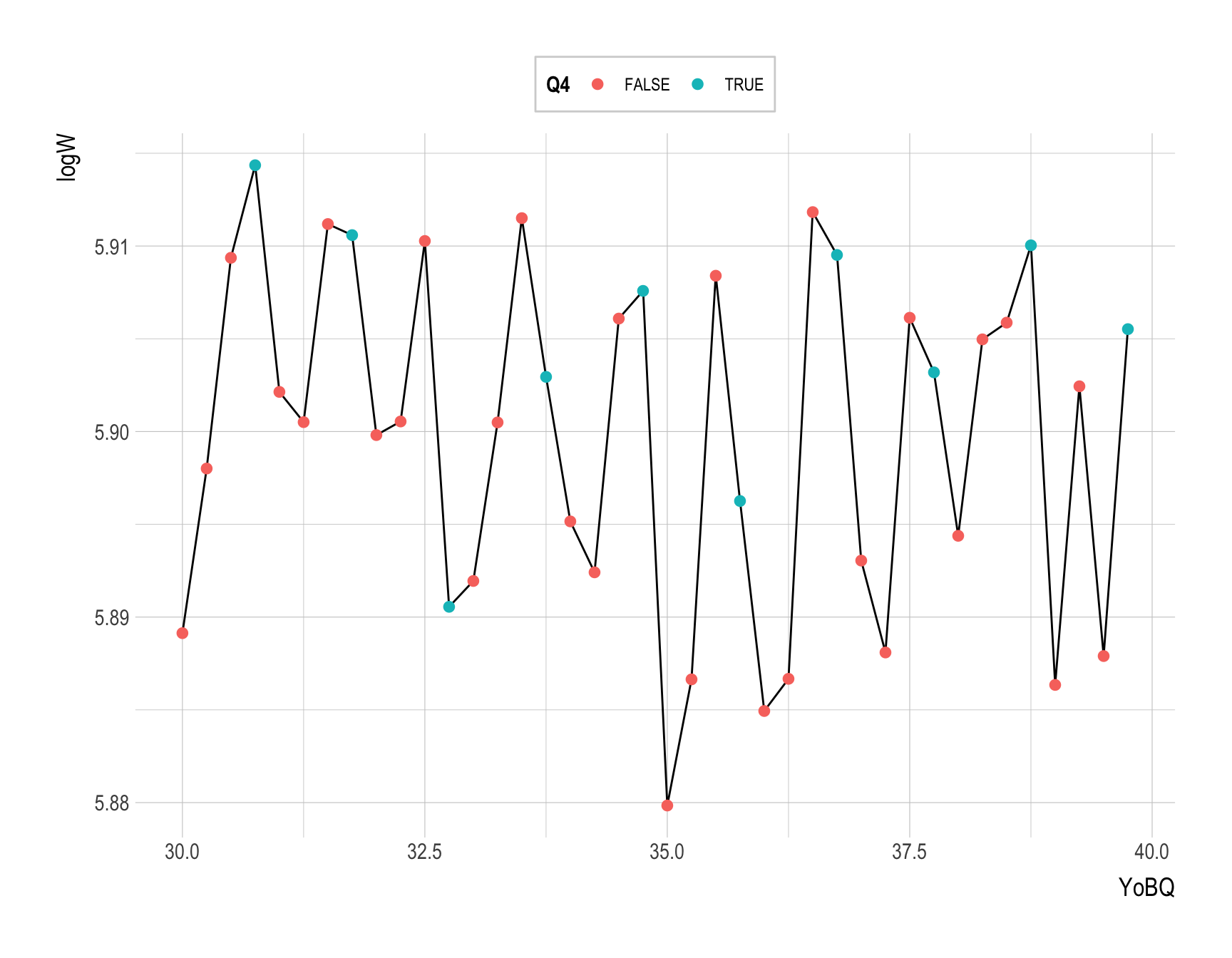
Q4c.
Provide a comment on the visulazations in Q4a and Q4b
Answer:
Question 5
- The following is the data.frame for Question 5.
holiday_movies <- read_csv("https://bcdanl.github.io/data/holiday_movies.csv")- The data.frame holiday_movies comes from the Internet Movie Database (IMDb).
Variable description
tconst: alphanumeric unique identifier of the title
title_type: the type/format of the title
- (movie, video, or tvMovie)
primary_title: the more popular title / the title used by the filmmakers on promotional materials at the point of release
simple_title: the title in lowercase, with punctuation removed, for easier filtering and grouping
year: the release year of a title
runtime_minutes: primary runtime of the title, in minutes
average_rating: weighted average of all the individual user ratings on IMDb
num_votes: number of votes the title has received on IMDb (titles with fewer than 10 votes were not included in this dataset)
- The following is the data.frame, holiday_movies.
Code
rmarkdown::paged_table(holiday_movies,
                       options = list(rows.print = 20,
                                      cols.print = 6,
                                      pages.print = 0,
                                      paged.print = F
                                      ))
Code
rmarkdown::paged_table(holiday_movies |> select(primary_title),
                       options = list(rows.print = 20,
                                      cols.print = 6,
                                      pages.print = 0,
                                      paged.print = F
                                      ))
Code
rmarkdown::paged_table(holiday_movies |> select(simple_title, year),
                       options = list(rows.print = 20,
                                      cols.print = 6,
                                      pages.print = 0,
                                      paged.print = F
                                      ))
Code
rmarkdown::paged_table(holiday_movies |> select(runtime_minutes:num_votes),
                       options = list(rows.print = 20,
                                      cols.print = 6,
                                      pages.print = 0,
                                      paged.print = F
)) nrow(holiday_movies)[1] 2265ncol(holiday_movies)[1] 8unique(holiday_movies$title_type)[1] "movie" "tvMovie" "video" length(unique(holiday_movies$primary_title))[1] 2081unique(holiday_movies$primary_title)[1:50] [1] "Sailor's Holiday" "The Devil's Holiday"
[3] "Holiday" "Holiday of St. Jorgen"
[5] "Sin Takes a Holiday" "Sinners' Holiday"
[7] "Husband's Holiday" "Beggar's Holiday"
[9] "Cowboy Holiday" "Death Takes a Holiday"
[11] "College Holiday" "Mad Holiday"
[13] "Stolen Holiday" "Angel's Holiday"
[15] "Dangerous Holiday" "Every Day's a Holiday"
[17] "Bank Holiday" "A Christmas Carol"
[19] "Crime Takes a Holiday" "Tropic Holiday"
[21] "Inspector Hornleigh on Holiday" "Christmas in July"
[23] "Holiday Inn" "Hoosier Holiday"
[25] "Christmas Holiday" "Knickerbocker Holiday"
[27] "Christmas in Connecticut" "Strange Holiday"
[29] "Holiday in Mexico" "Perilous Holiday"
[31] "Blondie's Holiday" "Bush Christmas"
[33] "Christmas Eve" "Hoppy's Holiday"
[35] "Holiday Camp" "Summer Holiday"
[37] "Holidays in Hell" "Holiday Affair"
[39] "Holiday in Havana" "Johnny Holiday"
[41] "Holiday Rhythm" "Last Holiday"
[43] "Holiday Week" "Holiday for Sinners"
[45] "Roman Holiday" "Monsieur Hulot's Holiday"
[47] "White Christmas" "Cinerama Holiday"
[49] "Holiday for Henrietta" "Holiday Island" length(unique(holiday_movies$simple_title))[1] 2073unique(holiday_movies$simple_title)[1:50] [1] "sailors holiday" "the devils holiday"
[3] "holiday" "holiday of st jorgen"
[5] "sin takes a holiday" "sinners holiday"
[7] "husbands holiday" "beggars holiday"
[9] "cowboy holiday" "death takes a holiday"
[11] "college holiday" "mad holiday"
[13] "stolen holiday" "angels holiday"
[15] "dangerous holiday" "every days a holiday"
[17] "bank holiday" "a christmas carol"
[19] "crime takes a holiday" "tropic holiday"
[21] "inspector hornleigh on holiday" "christmas in july"
[23] "holiday inn" "hoosier holiday"
[25] "christmas holiday" "knickerbocker holiday"
[27] "christmas in connecticut" "strange holiday"
[29] "holiday in mexico" "perilous holiday"
[31] "blondies holiday" "bush christmas"
[33] "christmas eve" "hoppys holiday"
[35] "holiday camp" "summer holiday"
[37] "holidays in hell" "holiday affair"
[39] "holiday in havana" "johnny holiday"
[41] "holiday rhythm" "last holiday"
[43] "holiday week" "holiday for sinners"
[45] "roman holiday" "monsieur hulots holiday"
[47] "white christmas" "cinerama holiday"
[49] "holiday for henrietta" "holiday island" length(unique(holiday_movies$year))[1] 91unique(holiday_movies$year) [1] 1929 1930 1931 1934 1936 1937 1938 1939 1940 1942 1943 1944 1945 1946 1947
[16] 1948 1949 1950 1951 1952 1953 1954 1955 1957 1958 1959 1960 1963 1961 1964
[31] 1965 1966 1967 1969 1970 1971 1972 1973 1974 1975 1976 1977 1978 1979 1981
[46] 1980 1983 1984 1986 1985 1987 1988 1989 1990 1991 1993 1992 1994 1995 1997
[61] 1996 1962 1998 1968 2000 1999 2001 2004 2002 1982 2008 2003 1956 2007 2005
[76] 2006 2016 2014 2019 2018 2020 2021 2011 2023 2017 2009 2022 2012 2015 2010
[91] 2013unique(holiday_movies$runtime_minutes) [1] 58 80 91 83 81 60 70 56 79 86 71 76 69 59 95 78 90 67
[19] 100 65 93 85 101 61 128 89 NA 87 73 92 88 82 72 118 114 120
[37] 119 105 103 125 75 107 68 84 96 25 94 26 110 98 22 113 97 48
[55] 109 24 133 127 49 123 43 50 104 40 102 30 55 46 44 53 115 132
[73] 23 64 52 158 145 130 57 66 45 47 51 29 27 63 7 99 18 54
[91] 112 6 9 33 136 5 39 28 15 122 74 35 41 10 20 152 106 220
[109] 31 4 1 37 17 146 140 77 150 141 42 3 121 111 21 12 172 108
[127] 2 34 180 131 11 160 286 165 16 135 288 126 117 36 213unique(holiday_movies$average_rating) [1] 5.4 6.0 6.3 7.4 6.1 6.4 5.6 4.8 6.9 5.7 5.8 6.2 7.5 6.5 7.7
[16] 5.5 6.8 7.3 6.7 5.3 6.6 5.9 7.1 8.1 8.0 7.6 8.3 3.5 4.4 7.2
[31] 4.2 8.2 7.8 4.7 7.9 5.2 5.0 8.9 5.1 7.0 4.9 3.1 4.0 2.0 8.5
[46] 4.3 8.7 2.1 2.4 4.1 2.2 2.9 4.6 3.9 3.6 4.5 8.6 2.7 3.8 3.2
[61] 8.4 3.7 9.0 9.4 9.1 9.2 9.3 3.3 3.4 1.5 10.0 1.4 2.8 8.8 9.9
[76] 9.8 2.6 9.5 1.6 1.3 1.7 1.8 3.0 1.0 2.3- The following is another data.frame holiday_movie_genres that is related with the data.frame holiday_movies:
holiday_movie_genres <- read_csv("https://bcdanl.github.io/data/holiday_movie_genres.csv")Code
rmarkdown::paged_table(holiday_movie_genres,
                       options = list(rows.print = 20,
                                      cols.print = 6,
                                      pages.print = 0,
                                      paged.print = F
)) - The data.frame holiday_movie_genres include up to three genres associated with the titles that appear in the data.frame.
unique(holiday_movie_genres$genres) [1] "Comedy" "Drama" "Romance" "Adventure" "Crime"
[6] "Western" "Fantasy" "Musical" "Mystery" "Family"
[11] "Action" "Music" "Film-Noir" "History" "War"
[16] "Thriller" NA "Documentary" "Animation" "Sci-Fi"
[21] "Horror" "Short" "Biography" "Sport" "Talk-Show"
[26] "News" "Reality-TV" Variable description
- tconst: alphanumeric unique identifier of the title
- genres: genres associated with the title, one row per genre
Q5a. [Out of Coverage in Spring 2024, DANL 200-02]
- Provide the R code to generate the data.frame, holiday_movie_with_genres, which combines the two data.frames, holiday_movies and holiday_movie_genres:
Answer:
Code
holiday_movies_with_genres <- holiday_movie_genres |>
left_join(holiday_movies)- The following shows the first four variables in holiday_movie_with_genres:
Code
rmarkdown::paged_table(holiday_movies_with_genres,
                       options = list(rows.print = 20,
                                      cols.print = 6,
                                      pages.print = 0,
                                      paged.print = F
                                      ))
Q5b.
Provide the R code to see how the summary statistics—mean, median, standard deviation, minimum, maximum, first and third quartiles—of average_rating and num_votes varies by popular genres and title_type.
- Consider only the five popular genres, which are selected in terms of the number of titles for each genre.
- Removes the video type of the titles when calculating the summary statistics.
Answer:
Code
popular_genres <- holiday_movies_with_genres |>
  group_by(genres) |>
  count() |>
  ungroup() |>
  slice_max(n, n = 5)

holiday_movies_with_genres |>
  filter(genres %in% popular_genres$genres,
         title_type != 'video') |>
  group_by(genres, title_type) |>
  skim(average_rating, num_votes)
Q5c.
- Provide R code to recreate the ggplot figure illustrating how the relationship between log10(num_votes) and average_rating varies by the popular genres and title_type.
- The five popular genres are selected in terms of the number of titles for each genre.
- The video type of the titles are removed in the ggplot figure.
Answer:
Code
popular_genres <- holiday_movies_with_genres |>
  group_by(genres) |>
  count() |>
  ungroup() |>
  slice_max(n, n = 5)

holiday_movies_with_genres |>
  filter(genres %in% popular_genres$genres,
         title_type != 'video') |>
  group_by(genres) |>
  mutate(mean_rating = mean(average_rating, na.rm = T)) |>
  ggplot(aes(y = average_rating, x = log10(num_votes))) +
  geom_point(alpha = .2) +
  geom_smooth(aes(color = genres),
              method = lm) +
  # coord_cartesian(ylim = c(5,7)) +
  facet_grid(title_type~ genres, scales = "free")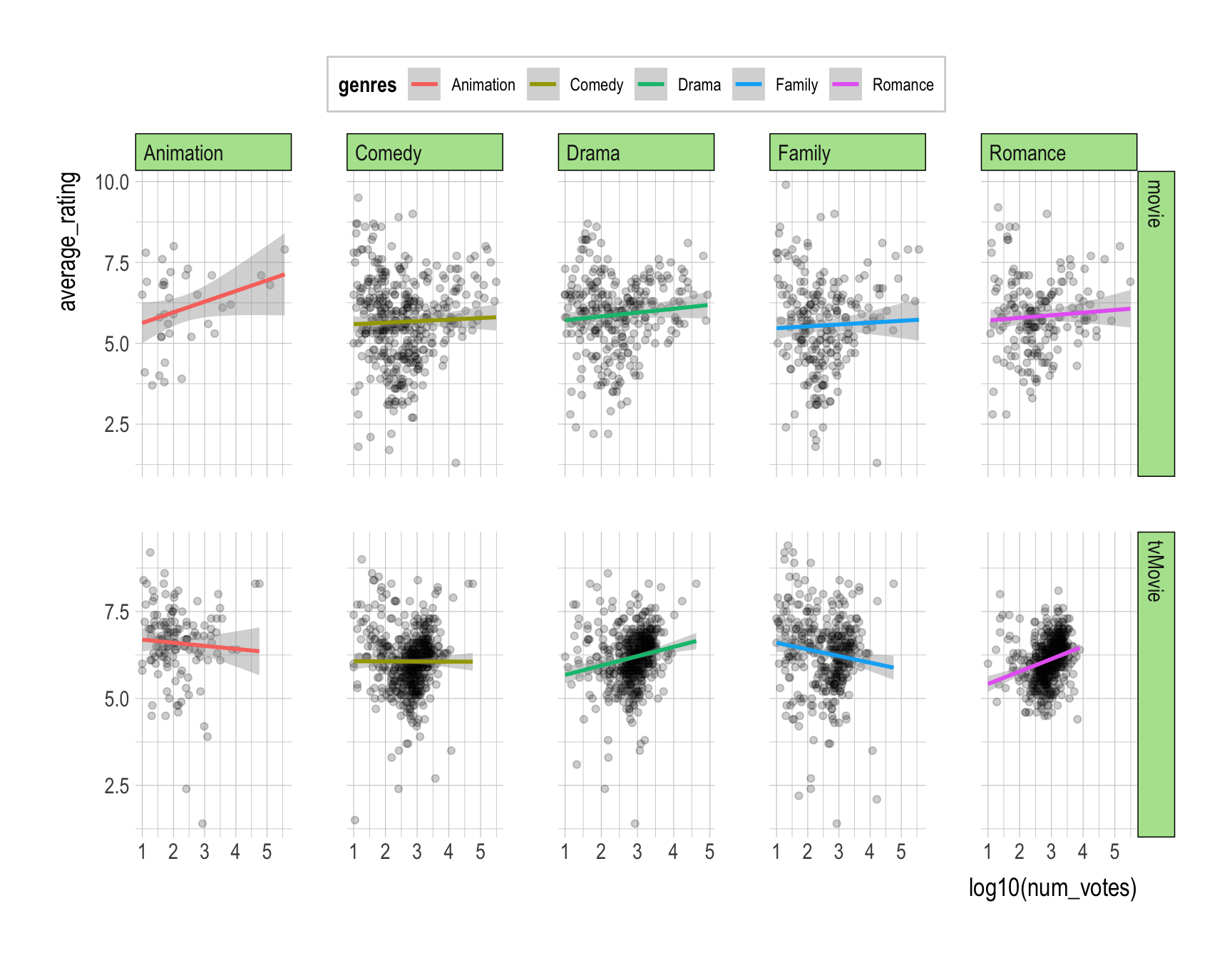
Q5d.
- Provide a comment to illustrate how the relationship between log10(num_votes) and average_rating varies by the popular genres and title_type.
Answer:
Q5e.
Provide R code to recreate the ggplot figure illustrating the annual trend of the share of number of movies by popular genre from year 1975 to 2022.
- For genres that are not popular, categorize them as “Other”.
- Consider changing the order of categories in genres.
Answer:
Code
df <- holiday_movies_with_genres |>
  mutate(genres = ifelse( !(genres %in% popular_genres$genres), "Other", genres )) |>
  group_by(year, genres) |>
  count() |>
  filter(year >= 1975, year <= 2022)

ggplot(df) +
  geom_col(aes(x = year, y = n,
               fill = fct_reorder2(genres, year, n)), # fct_reorder2() is out of our coverage
           position = 'fill',
           width = rel(1.25), # width = ... is out of our coverage
           color = 'black') +
  labs(y = "Share of number of movies by genre",  # labs() is not necessary
       fill = "genres") +
  scale_fill_brewer(palette = "Accent") # out of our coverage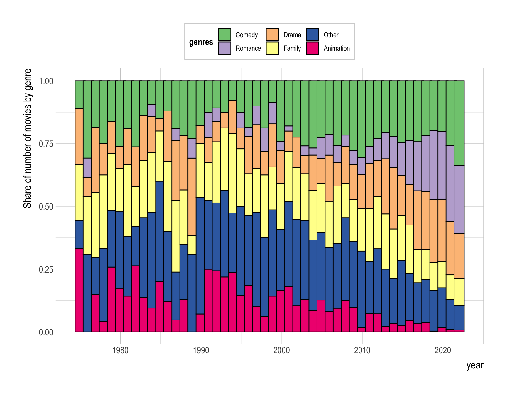
Q5f.
Provide a comment to illustrate the annual trend of (1) the share of number of movies by popular genre from year 1975 to 2022.
- Which genre has become more popular since 2010?
Answer:
Q5g.
Add the following two variables—christmas and holiday—to the data.frame holiday_movies_with_genres:
christmas:
- TRUE if the simple_title includes “christmas”, “xmas”, “x mas”
- FALSE otherwise
holiday:
- TRUE if the simple_title includes “holiday”
- FALSE otherwise
Answer:
Code
holiday_movies_with_genres <- holiday_movies_with_genres |>
  mutate(christmas = ifelse(str_detect(simple_title, "christmas") |
                              str_detect(simple_title, "xmas") |
                              str_detect(simple_title, "x mas"),
                            T, F),
         holiday = ifelse(str_detect(simple_title, "holiday"),
                            T, F),
         )
Q5h.
- Provide R code to recreate the ggplot figure illustrating the annual trend of (1) the number of movie titles with “holiday” varies by christmas.
Answer:
Code
df <- holiday_movies_with_genres |>
  group_by(year, christmas, holiday) |>
  count()

ggplot(df, aes(x = year, y = n, color = holiday)) +
  geom_smooth() +
  geom_point(alpha = .33) +
  facet_wrap(christmas~., scales = "free")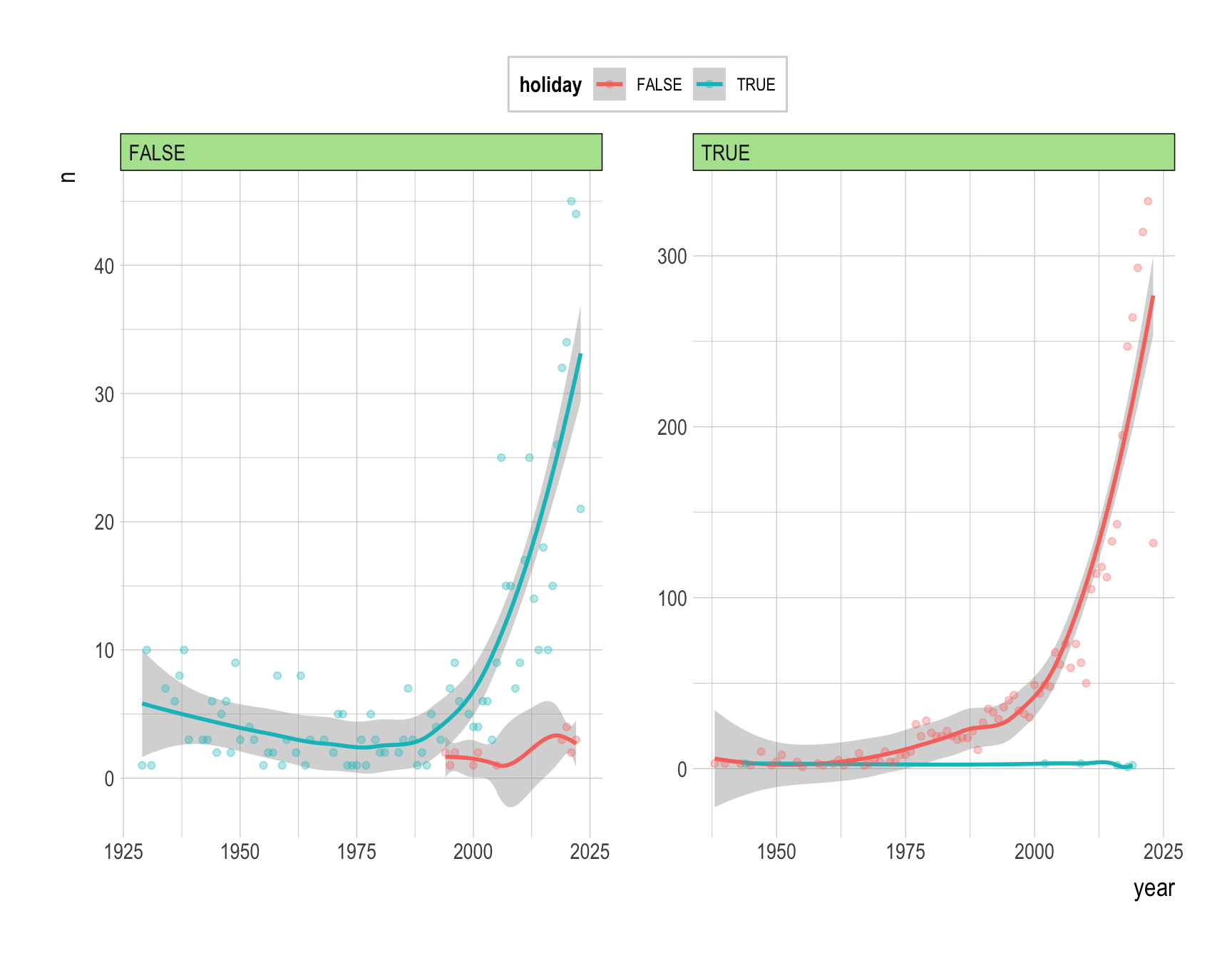
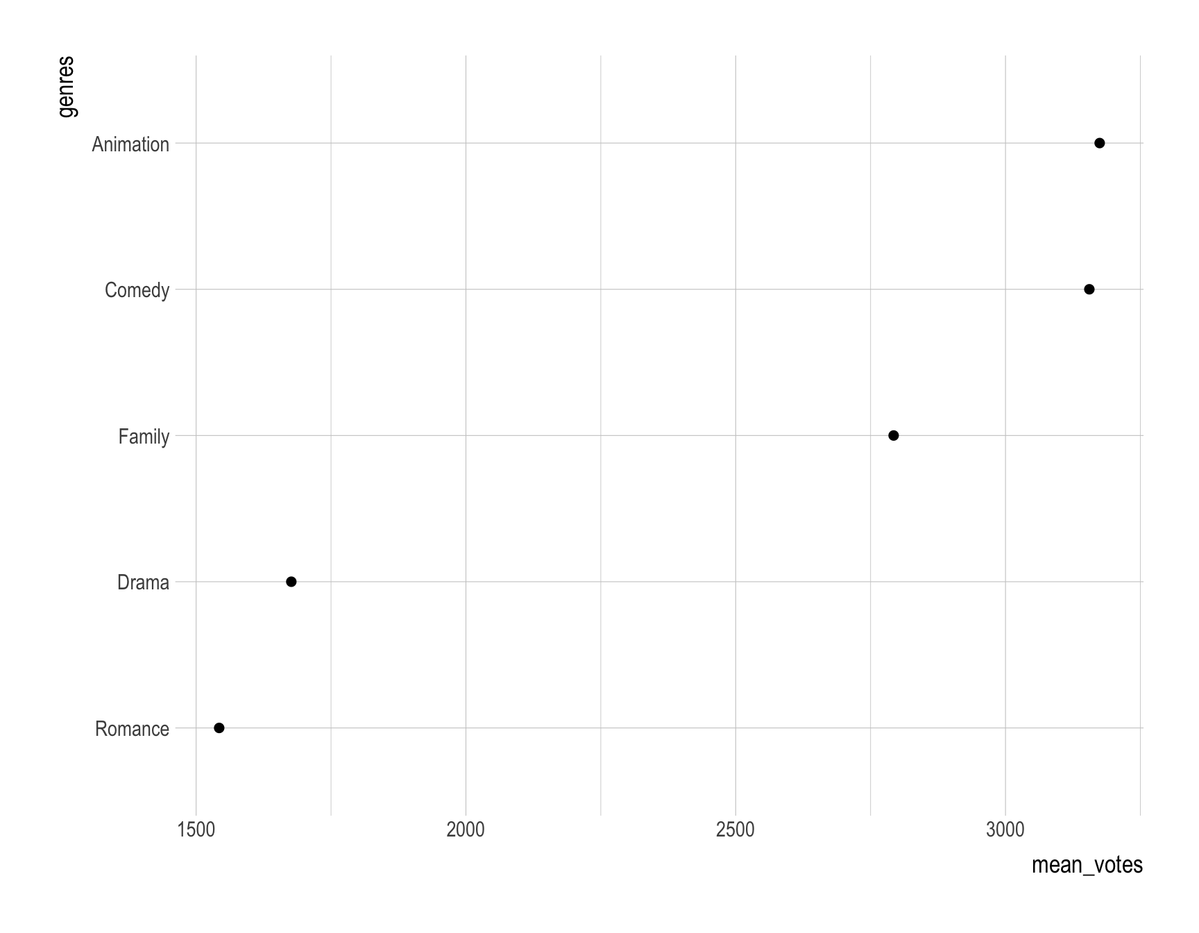
Q5i.
- Provide R code to recreate the ggplot figure illustrating how the mean value of num_votes varies by the popular genres for the titles with “christmas”.
Answer:
Code
df <- holiday_movies_with_genres |>
  filter(genres %in% popular_genres$genres) |>
  group_by(genres, christmas) |>
  summarise(mean_rating = mean(average_rating),
            mean_votes = mean(num_votes)) |>
  filter(christmas == T)

ggplot(df, aes(x = mean_votes, y = fct_reorder(genres, mean_votes),
             )) +
  geom_point(size = 2) +
  labs(y = "genres")  # labs() is not necessary