1 + 1[1] 2Data-Driven Mastery: Unlocking Business Potential
About this project 👏
1 + 1[1] 2The data.frame mpg contains a subset of the fuel economy data that the EPA makes available on https://fueleconomy.gov/. It contains only models which had a new release every year between 1999 and 2008 - this was used as a proxy for the popularity of the car. 🚘
mpg <- ggplot2::mpgskim(mpg) %>%
select(-n_missing)| Name | mpg |
| Number of rows | 234 |
| Number of columns | 11 |
| _______________________ | |
| Column type frequency: | |
| character | 6 |
| numeric | 5 |
| ________________________ | |
| Group variables | None |
Variable type: character
| skim_variable | complete_rate | min | max | empty | n_unique | whitespace |
|---|---|---|---|---|---|---|
| manufacturer | 1 | 4 | 10 | 0 | 15 | 0 |
| model | 1 | 2 | 22 | 0 | 38 | 0 |
| trans | 1 | 8 | 10 | 0 | 10 | 0 |
| drv | 1 | 1 | 1 | 0 | 3 | 0 |
| fl | 1 | 1 | 1 | 0 | 5 | 0 |
| class | 1 | 3 | 10 | 0 | 7 | 0 |
Variable type: numeric
| skim_variable | complete_rate | mean | sd | p0 | p25 | p50 | p75 | p100 | hist |
|---|---|---|---|---|---|---|---|---|---|
| displ | 1 | 3.47 | 1.29 | 1.6 | 2.4 | 3.3 | 4.6 | 7 | ▇▆▆▃▁ |
| year | 1 | 2003.50 | 4.51 | 1999.0 | 1999.0 | 2003.5 | 2008.0 | 2008 | ▇▁▁▁▇ |
| cyl | 1 | 5.89 | 1.61 | 4.0 | 4.0 | 6.0 | 8.0 | 8 | ▇▁▇▁▇ |
| cty | 1 | 16.86 | 4.26 | 9.0 | 14.0 | 17.0 | 19.0 | 35 | ▆▇▃▁▁ |
| hwy | 1 | 23.44 | 5.95 | 12.0 | 18.0 | 24.0 | 27.0 | 44 | ▅▅▇▁▁ |
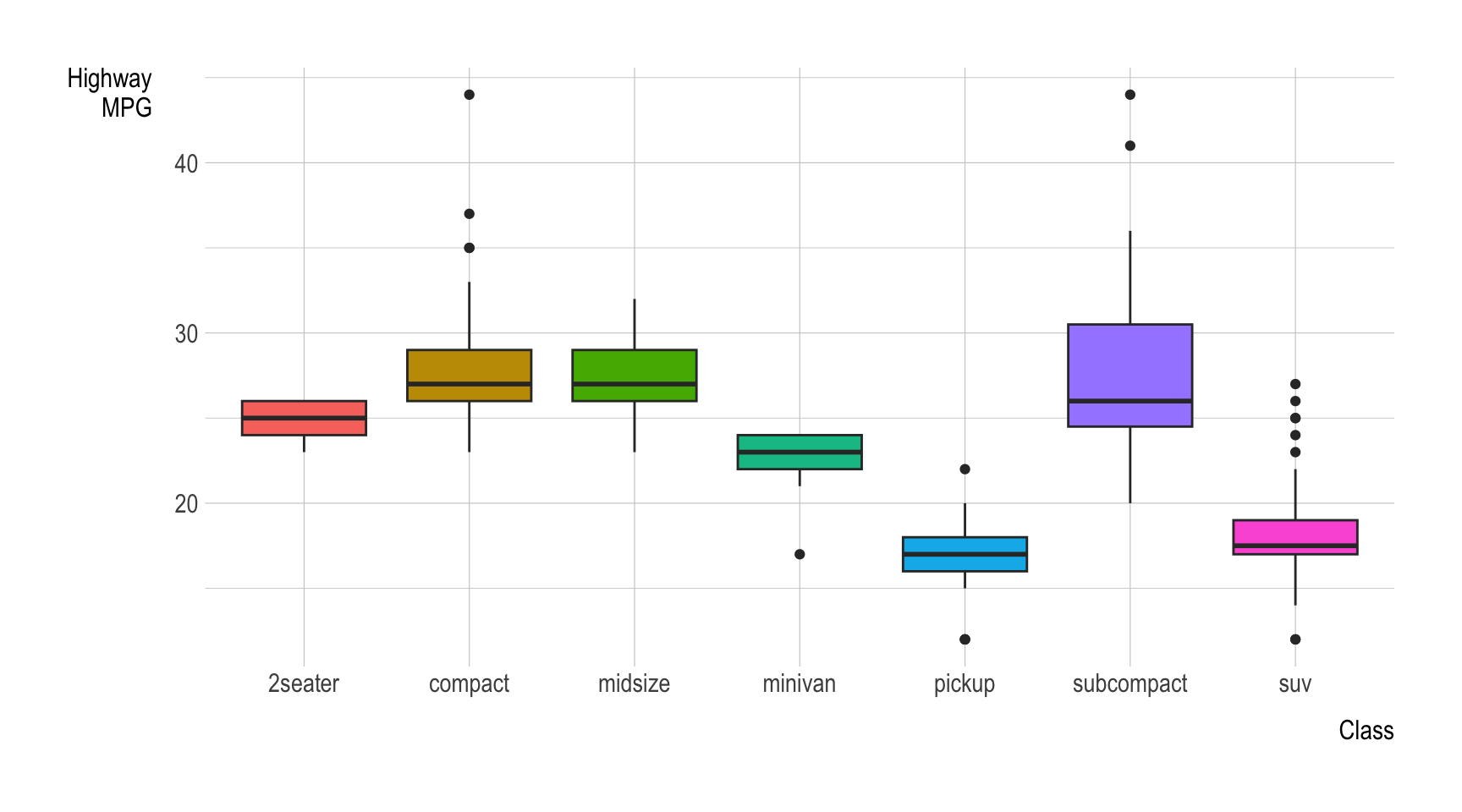
The following boxplot shows how the distribution of highway MPG (hwy) varies by a type of cars (class) 🚙 🚚 🚐.
ggplot(data = mpg) +
  geom_boxplot(aes(x = class, y = hwy, fill = class),
               show.legend = F) +
  labs(x = "Class", y = "Highway\nMPG")