Lecture 8

Data Visualization II: Relationships and Time Trends

Byeong-Hak Choe

SUNY Geneseo

November 1, 2026

๐Ÿ”— Relationships between variables

๐Ÿงฉ The same grammar supports a new question

  • We have used data, mappings in aes(), and a geom layer to show distributions and compare groups.
  • Now the question is: How is engine size related to highway fuel economy?
  • A scatterplot maps two numeric variables to horizontal and vertical positions.
Part of the plot What stays familiar What changes here
data = mpg The data frame We keep the same vehicle rows
mapping = aes(...) Variables control visual features Both x and y contain numeric variables
geom_*() A layer draws the data geom_point() draws a point for each row

๐Ÿ”ต A scatterplot places each row using two values

ggplot(data = mpg,
       mapping = aes(x = displ,
                     y = hwy)) +
  geom_point() +
  labs(
    x = "Engine size (liters)",
    y = "Highway fuel economy (mpg)"
  )
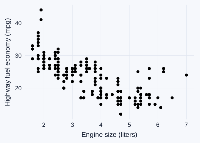
Scatterplot of engine size in liters and highway fuel economy in miles per gallon. Larger engines generally accompany lower highway fuel economy.

  • displ gives engine size in liters. hwy gives highway miles per gallon.
  • One point represents one vehicle in the dataset, as in our earlier mpg charts.

๐Ÿ‘€ Direction, shape, and unusual points

  • Direction: larger engines generally accompany lower highway mpg. We call this a negative association.
  • Shape and spread: the pattern may curve. Vehicles with similar engine sizes can have different highway mpg.
  • Unusual points: a vehicle far from the overall pattern deserves a closer look at its row and context.

โš ๏ธ Association and cause

  • A scatterplot describes how variables vary together in these observations.
  • Vehicles also differ in weight, design, and transmission. Those features may relate to both engine size and fuel economy.
  • Establishing a causal effect requires an appropriate study design and additional evidence. This chart alone cannot isolate the effect of changing engine size.

๐Ÿš™ Drive system adds a categorical variable

drv Drive system
f Front-wheel drive
r Rear-wheel drive
4 Four-wheel drive
  • These are the same categories used in our grouped histograms and boxplots.
  • We can distinguish them within the scatterplot to see where groups overlap.

๐ŸŽจ Mapped color identifies groups

library(ggthemes)

ggplot(data = mpg,
       mapping = aes(x = displ,
                     y = hwy,
                     color = drv)) +
  geom_point(alpha = 0.5) +
  scale_color_tableau() +
  labs(
    x = "Engine size (liters)",
    y = "Highway fuel economy (mpg)",
    color = "Drive system"
  )
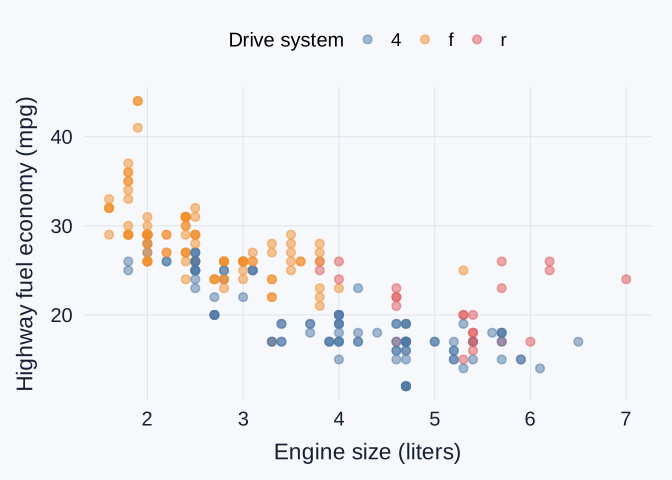
Scatterplot of engine size and highway mpg. Point color identifies drive system, and semitransparency helps reveal overlapping observations.

  • color = drv inside aes() maps groups to colors. scale_color_tableau() chooses those colors.
  • alpha = 0.5 makes points partly transparent. Overlapping points appear darker.

๐Ÿ–Œ๏ธ Mappings and fixed appearances

ggplot(data = mpg,
       mapping = aes(x = displ,
                     y = hwy)) +
  geom_point(color = "steelblue", alpha = 0.5)
Code Meaning
aes(color = drv) Let a variable determine each pointโ€™s color
geom_point(color = "steelblue") Give every point the same chosen color
  • A variable belongs inside aes() when its values should control a visual feature.
  • A fixed appearance belongs outside aes(). A color name inside aes() can create an unintended legend.

๐ŸชŸ Familiar facets separate the groups

ggplot(data = mpg,
       mapping = aes(x = displ,
                     y = hwy)) +
  geom_point(alpha = 0.5) +
  facet_wrap(~ drv)

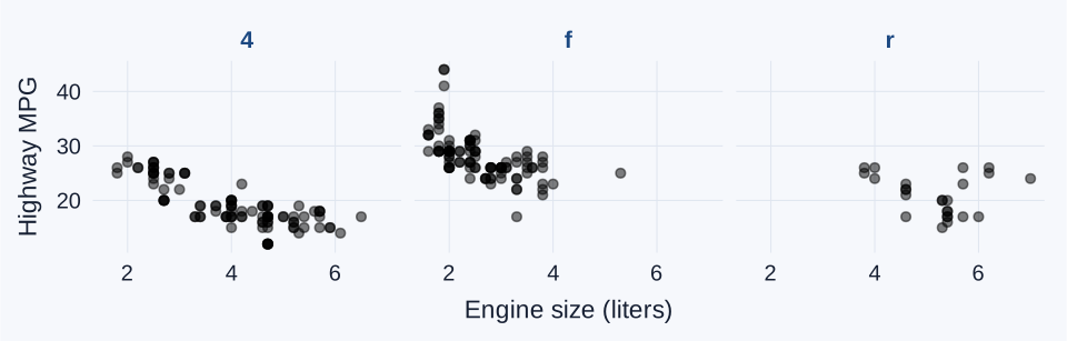
Three scatterplot panels compare engine size and highway mpg within four-wheel, front-wheel, and rear-wheel drive. All panels share the same axis scales.

  • Familiar facet_wrap(~ drv) panels use shared axes, just as in our histograms. The groups also cover different engine-size ranges.

๐Ÿ“‰ A fitted line adds a summary layer

ggplot(data = mpg,
       mapping = aes(x = displ,
                     y = hwy)) +
  geom_point(alpha = 0.5) +
  geom_smooth(
    method = "lm", se = FALSE
  ) +
  labs(
    x = "Engine size (liters)",
    y = "Highway fuel economy (mpg)"
  )
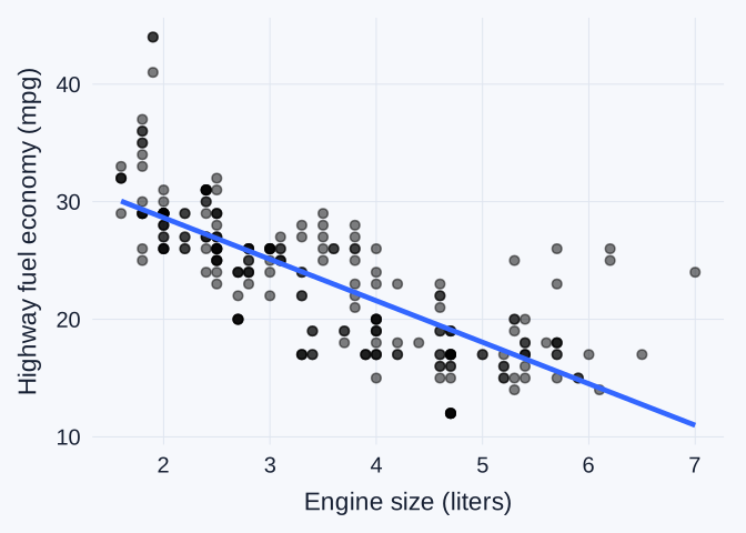
Engine size and highway mpg scatterplot with a fitted straight line summarizing the overall downward pattern. Points vary around the line.

  • + adds another layer to the same plot. method = "lm" requests a fitted straight line.
  • se = FALSE hides the shaded uncertainty band. The line summarizes the overall direction, while the points show variation around it.

โœ๏ธ Classwork 14: Relationships

  • Questions 1โ€“5 apply points, mapped color, facets, and a fitted line to city and highway mpg, comparing the two model years.
  • The group-comparison questions in Classwork 14 begin at Question 2. The log-transformation classwork follows the next lecture section.

๐ŸŒ Log transformations and relationships

๐ŸŒ Historical country data

Country GDP per person Life expectancy
Afghanistan 974.6 43.8
Albania 5937.0 76.4
Algeria 6223.4 72.3
Angola 4797.2 42.7
  • Each row represents one country in 2007, with 142 countries in this dataset.
  • gdpPercap is GDP per person in inflation-adjusted dollars, a measure of economic output per person rather than personal salary.
  • lifeExp is life expectancy at birth in years. These historical observations do not describe current conditions.

๐Ÿ“ฅ Importing the country data

gapminder_2007 <- read_tsv(
  "https://bcdanl.github.io/data/gapminder.tsv"
) |>
  filter(year == 2007)
  • read_tsv() reads a file whose columns have tab separators, rather than comma separators.
  • filter(year == 2007) keeps a single year, so each country contributes one observation.
  • The plotting grammar stays the same when we replace mpg with a different data frame.

๐Ÿงฎ Logarithms express multiplicative differences

Original value \(x\) \(\log_{10}(x)\) Why
100 2 \(10^2 = 100\)
1,000 3 \(10^3 = 1{,}000\)
10,000 4 \(10^4 = 10{,}000\)
  • Equal tenfold increases become equal one-unit steps after log10().
  • In R, log10(x) uses base 10. log(x) uses the natural-log base \(e \approx 2.718\).
log10(c(100, 1000, 10000))  # 2, 3, 4

๐Ÿ“Š A log transformation changes the spacing

Original GDP
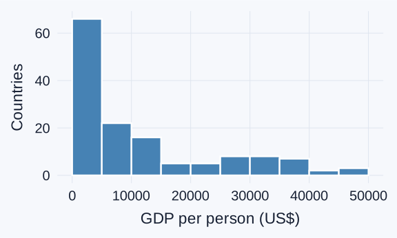
Histogram of original GDP per person in 2007, with many countries at the lower end and a long right tail.

mapping = aes(x = gdpPercap)

Logged GDP

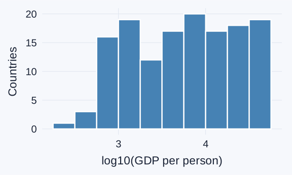
Histogram of base-10 log GDP per person for the same 142 countries, with more space between lower-GDP values and a compressed upper tail.

mapping = aes(x = log10(gdpPercap))
  • The same 142 countries remain in both plots. Logging preserves their order but changes the distances between values.

๐ŸŒ GDP and life expectancy on two scales

Original GDP
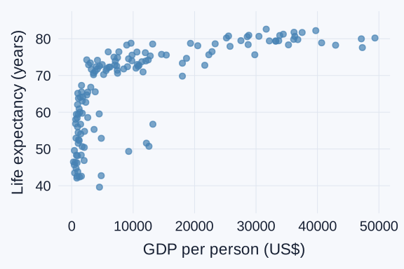
Scatterplot of life expectancy against original GDP per person in 2007. Many lower-GDP countries crowd together on the left.

Logged GDP

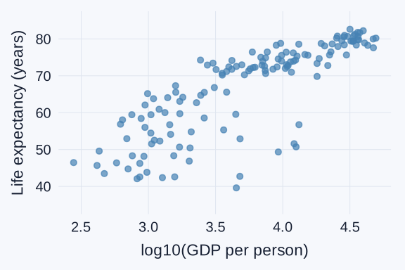
Scatterplot of life expectancy against base-10 log GDP per person, making differences among lower-GDP countries easier to distinguish.

  • Higher GDP per person generally accompanies higher life expectancy in these observations. The scale change does not establish a causal relationship.

๐Ÿงฉ A transformation can go inside aes()

ggplot(data = gapminder_2007,
       mapping = aes(x = log10(gdpPercap),
                     y = lifeExp)) +
  geom_point()
  • log10(gdpPercap) calculates the horizontal positions from the GDP values.
  • lifeExp stays in its original units: years.
  • The plot uses transformed positions without replacing the original gdpPercap column.

โš ๏ธ Log transformations require positive values

  • For the real-valued logarithms we use here, inputs must be positive. log10(0) returns -Inf, and negative inputs produce NaN.
  • A value that looks less extreme after logging still deserves attention. The transformation changes the display rather than correcting a data error.
  • Adding 1 automatically changes the transformation and its meaning. First investigate what any zero or negative value represents.

โœ๏ธ Classwork 15: Log transformations

  • Compare population and life expectancy on original and logged population axes.
  • Focus on how the spacing changes and which country differences become easier to see.

๐Ÿ—“๏ธ Stock-price rows identify a company and a date

Date Company ticker Closing price (US$)
2026-10-01 AAPL 330.32
2026-10-01 NVDA 230.86
2026-10-02 AAPL 333.69
2026-10-02 NVDA 233.95
  • Each row represents one company on one trading day in October 2026.
  • AAPL identifies Apple, and NVDA identifies NVIDIA. Close gives the closing price per share in US dollars.
  • A line chart lets us follow these observations in chronological order.

๐Ÿ—“๏ธ Preparing dates and selecting companies

tech_october <- read_csv(
  "https://bcdanl.github.io/data/tech_stocks_2026_10.csv"
) 

tech_two <- tech_october |>
  filter(Ticker %in% c("AAPL", "NVDA"))

apple_october <- tech_two |>
  filter(Ticker == "AAPL")
  • as.Date() converts a value such as "2026-10-01" into Rโ€™s Date type. read_csv() may already recognize this format.
  • %in% checks membership in a set. Here it keeps two companies, and the final filter() keeps only Apple.

๐Ÿ“ˆ Points and a line show one companyโ€™s history

ggplot(data = apple_october,
       mapping = aes(x = Date,
                     y = Close)) +
  geom_line(color = "steelblue") +
  geom_point(color = "steelblue") +
  labs(
    x = "Date in October 2026",
    y = "Closing price (US$/share)"
  )
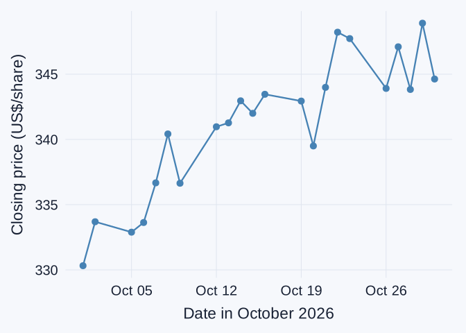
Points and a line show Apple's closing share price across trading days in October 2026, connecting observations in date order.

  • geom_point() marks the observed values. geom_line() connects them in x-axis order.
  • The file contains trading days. A connecting segment does not provide an observed closing price for every calendar day.

โš ๏ธ One line mixes the two companies

# Incorrect grouping
ggplot(data = tech_two,
       mapping = aes(x = Date,
                     y = Close)) +
  geom_line(color = "steelblue") +
  labs(
    x = "Date",
    y = "Closing price (US$/share)"
  )
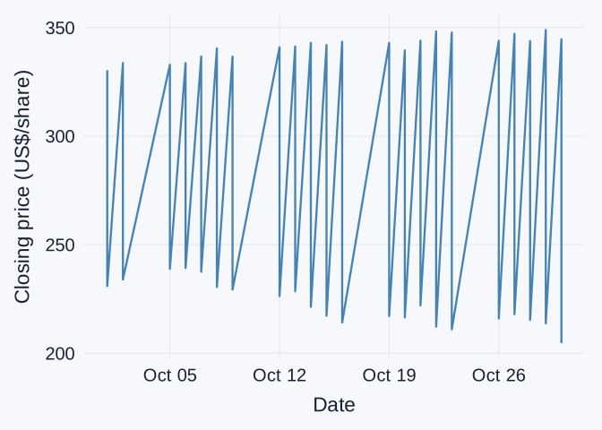
Incorrect plot joins Apple and NVIDIA prices as a single series, creating artificial jumps between companies on the same dates.

  • The combined data have two observations on each date, one per company.
  • This code connects the observations as one group, producing jumps between unrelated company prices.

๐Ÿงต Mapped color separates the company lines

ggplot(data = tech_two,
       mapping = aes(x = Date,
                     y = Close,
                     color = Ticker,
                     linetype = Ticker)) +
  geom_line(linewidth = 1) +
  scale_color_tableau() +
  labs(
    x = "Date",
    y = "Closing price (US$/share)",
    color = "Company",
    linetype = "Company"
  )
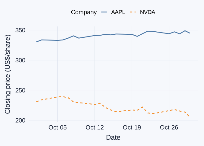
Separate Apple and NVIDIA price lines over October 2026. Both color and line type distinguish the companies.

  • Mapping the categorical Ticker variable to color creates a separate line for each company.
  • linetype = Ticker also distinguishes the companies when colors are hard to tell apart.

๐ŸชŸ Explicit grouping works with facets

ggplot(data = tech_two,
       mapping = aes(x = Date,
                     y = Close,
                     group = Ticker)) +
  geom_line(color = "steelblue") +
  facet_wrap(~ Ticker)
  • group = Ticker explicitly tells ggplot which rows belong to the same series.
  • facet_wrap(~ Ticker) places each companyโ€™s history in its own panel, with shared scales by default.
  • Fixed color controls appearance. The grouping and panel variables determine which observations appear together.

๐Ÿ”Ž A price chart has limits

  • A higher price per share does not establish that a company is larger or that its stock is a better investment.
  • Price levels do not directly compare percentage returns. That comparison requires a common starting point and an appropriate return calculation.
  • This historical chart covers October 2026. It cannot establish why a price moved or predict what happens next.

๐Ÿงญ Questions, variables, and ggplot layers

Question Variables Useful layer
How are values distributed? One numeric variable geom_histogram()
How do distributions differ across groups? Numeric + category geom_boxplot()
How do categories compare? Category counts or supplied values geom_bar() or geom_col()
How do variables vary together? Two numeric variables geom_point()
How does a quantity change through time? Date + numeric variable geom_line()
  • The data frame, aes(), and + remain familiar. The question guides the mappings and layers.

๐Ÿท๏ธ Labels for a project audience

labs(
  title = "Apple closing prices in October 2026",
  x = "Date",
  y = "Closing price (US$/share)",
  caption = "Source: Stock Analysis"
)
  • labs() changes displayed text without renaming the data columns.
  • For classwork and homework, recognize its purpose. You may omit it unless a question specifically requests labels.
  • Project charts need clear labels and units, plus a source and relevant time period. labs() is a convenient way to supply them.

๐Ÿ“ A finding needs evidence and a limitation

Worked example: city fuel economy by drive type

  • Finding: front-wheel-drive vehicles have higher median city fuel economy in this dataset.
  • Evidence: the median is 19 mpg, compared with 14 mpg for four-wheel-drive vehicles and 15 mpg for rear-wheel-drive vehicles.
  • Limitation: the groups differ in other vehicle characteristics. This comparison does not isolate a drive-system effect.

๐Ÿ“ Reproducible charts for the storytelling project

  • The R script should recreate the data preparation and charts from the original files, without depending on objects left in the Environment.
  • Each chart should support a question with an appropriate comparison. Its labels should make the observations and units clear.
  • A recommendation should stay within the evidence. State an important limitation and acknowledge any AI assistance according to course requirements.

โœ๏ธ Classwork 16: Time and a data story

  • Questions 1โ€“3 compare Microsoft and Meta trading-volume histories, then a short finding supported by evidence and a limitation.
  • The final interpretation prepares for the storytelling project.