Classwork 12

Color vs. Facet

Question 1. NBC Show Data

The nbc_show dataset comes from NBC’s TV pilots, containing information about television shows, their viewership metrics, and audience engagement.

library(tidyverse)
nbc_show <- read_csv("https://bcdanl.github.io/data/nbc_show.csv")

• Gross Ratings Points (GRP):
  Measures the estimated total viewership of a show — an indicator of its broadcast marketability.
  • 📺 A higher GRP suggests broader exposure and a more marketable program.
• Projected Engagement (PE):
  Captures how attentive and engaged viewers were after watching a show — a more suitable measure of audience engagement.
  • 🧠 After viewing, audiences take a short quiz testing order and detail recall.
    
  • This reflects their level of attention and retention (for both the show and its ads).
    
  • High PE values indicate strong viewer engagement.

Tasks

• 🤖 Task 1: Fill in the blanks in the provided ggplot() code chunk.
  
• 💬 Task 2: Add a brief comment describing the relationship between gross ratings points (GRP) and projected engagement (PE) varies by genre (Genre).

(1) Color

ggplot(__BLANK_1__ = nbc_show,
       mapping = aes(x = GRP,
                     y = PE,
                     __BLANK_2__ = Genre)) +
  geom_point() +
  geom_smooth(__BLANK_3__,
              se = FALSE)   # se = FALSE turns off the ribbon

(2) Facet

ggplot(data = nbc_show,
       mapping = aes(x = GRP,
                     y = PE)) +
  geom_point(show.legend = FALSE) +  # show.legend = FALSE turns of legend
  geom_smooth(method = __BLANK_1__,
              show.legend = FALSE,  # show.legend = FALSE turns of legend
              se = FALSE) +  # se = FALSE turns off the ribbon
  __BLANK_2___wrap(__BLANK_3__)

(3) Facet with Color

ggplot(data = nbc_show,
       mapping = aes(x = GRP,
                     y = PE,
                     color = __BLANK_1__)) +
  geom_point(show.legend = FALSE) +  # show.legend = FALSE turns of legend
  geom_smooth(method = __BLANK_2__,
              show.legend = FALSE,
              se = FALSE) +  # se = FALSE turns off the ribbon
  __BLANK_3___wrap(__BLANK_4__)

Question 2. GDP per capita and Life Expectancy

For Question 2, please install the R package gapminder before starting:

install.packages("gapminder")
??gapminder

The gapminder package provides a built-in dataset named gapminder, which contains country-level data on life expectancy, GDP per capita, and population across time.

Let’s assign it to a new object called df_gapminder:

df_gapminder <- gapminder::gapminder

Tasks

• 🤖 Task 1: Fill in the blanks in the provided ggplot() code chunk.
  
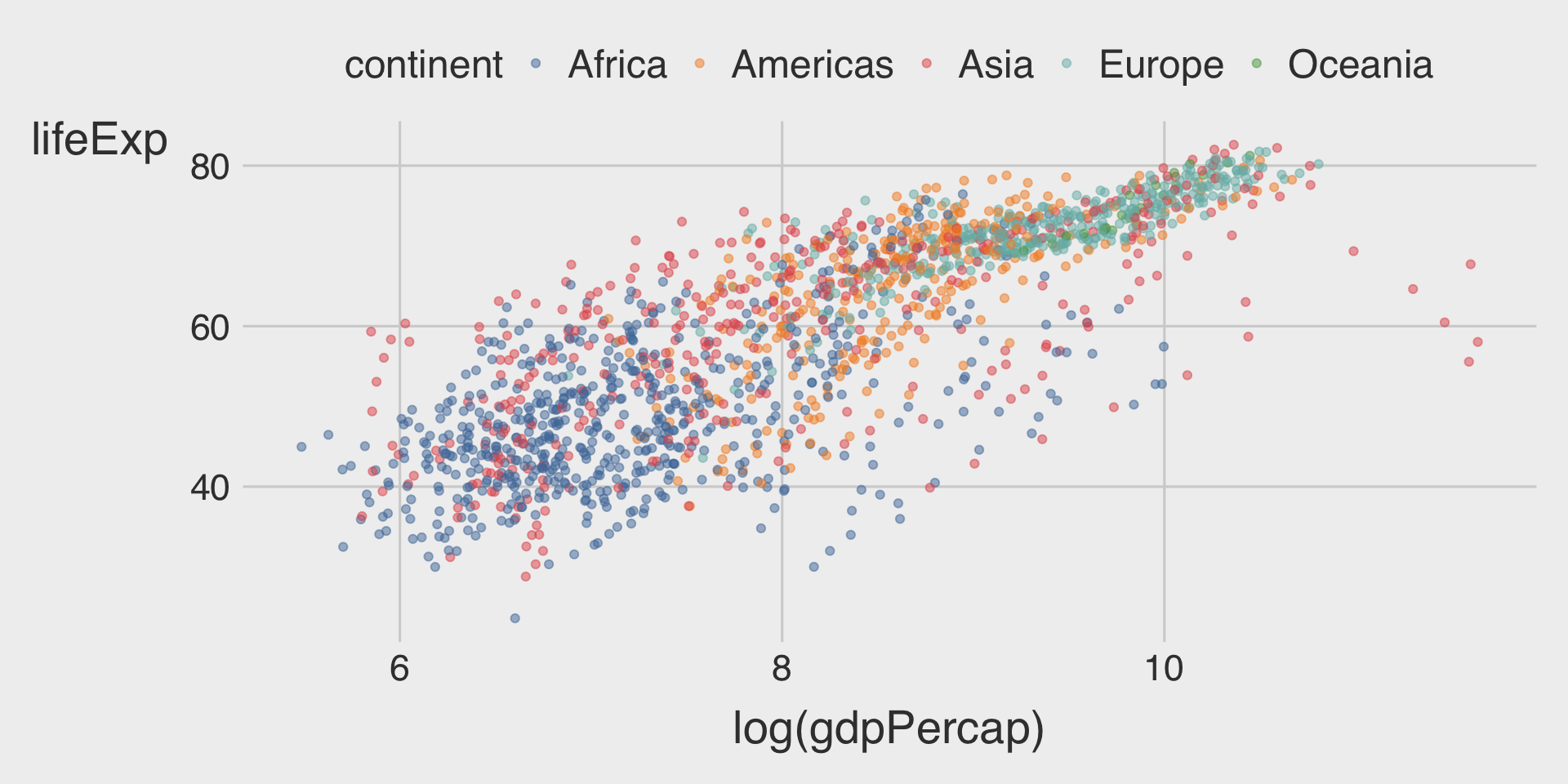
• 💬 Task 2: Add a brief comment describing the relationship between GDP per capita (gdpPercap) and life expectancy (lifeExp) varies by continents (continent).

(1) Color: Only Scatterplot

ggplot(__BLANK_1__ = df_gapminder,
       mapping = aes(__BLANK_2__ = log(gdpPercap),
                     __BLANK_3__ = lifeExp,
                     __BLANK_4__ = continent)) +  # different colors are used to distinguish continents
  geom_point(__BLANK_5__)  # Add transparency to reduce overplotting

(2) Color: Scatterplot with Fitted Line

ggplot(__BLANK_1__ = df_gapminder,
       mapping = aes(__BLANK_2__ = log(gdpPercap),
                     __BLANK_3__ = lifeExp,
                     __BLANK_4__ = continent)) +  # different colors are used to distinguish continents
  geom_point(__BLANK_5__) + # Add transparency to reduce overplotting
  geom___BLANK_6__(method = "lm")

(3) Facet: Scatterplot with Fitted Line

ggplot(__BLANK_1__ = df_gapminder,
       mapping = aes(__BLANK_2__ = log(gdpPercap),
                     __BLANK_3__ = lifeExp,
                     __BLANK_4__ = continent)) +
  geom_point(__BLANK_5__) +
  geom___BLANK_6__(method = "lm") +
  facet___BLANK_7__(~continent)

Question 3. Color vs. Facet

• What are the advantages of using faceting instead of the color aesthetic?
  
• What are the disadvantages?
  
• How might this trade-off change if you were working with a larger dataset?