df <- co2 |># Keep only country observations (drop regions / aggregates)# OWID country entries typically have a 3-letter ISO codefilter(!is.na(iso_code), nchar(iso_code) ==3) |># Keep useful sample years (adjust as you want)filter(year >=1990) |># Select a simple EKC-style set of variablesmutate(gdp_per_capita = gdp / population, .after = gdp ) |>select( iso_code, country, year, co2_per_capita, gdp_per_capita, population, energy_per_capita, # optional control primary_energy_consumption # optional control (can be NA a lot) ) |># Drop missing core variablesfilter(!is.na(co2_per_capita), !is.na(gdp_per_capita)) |># Create logs and squared log GDP per capitamutate(log_co2pc =log(co2_per_capita),log_gdppc =log(gdp_per_capita),log_gdppc2 = log_gdppc^2,log_pop =log(population),log_energy_pc =ifelse(!is.na(energy_per_capita) & energy_per_capita >0,log(energy_per_capita), NA) ) |># Keep rows with finite log outcomes/predictorsfilter(is.finite(log_co2pc), is.finite(log_gdppc), is.finite(log_gdppc2), is.finite(log_pop))# Convert to pdata.frame (panel format for plm)df_panel <-pdata.frame(df, index =c("iso_code", "year"))
Specify models
# Baseline (no optional controls)f_base <- log_co2pc ~ log_gdppc + log_gdppc2# Extended model (adds energy per capita; will drop rows with missing log_energy_pc)f_ext <- log_co2pc ~ log_gdppc + log_gdppc2 + log_energy_pc# --- Models (BASE) ---m1_pool <-plm(f_base, data = df_panel, model ="pooling") # pooled OLSm2_fe <-plm(f_base, data = df_panel, model ="within", effect ="individual") # country FEm3_twfe <-plm(f_base, data = df_panel, model ="within", effect ="twoways") # country FE + year FEm4_re <-plm(f_base, data = df_panel, model ="random", effect ="individual") # random effects# --- Models (EXTENDED) ---# (Optional) include energy per capita as a controlm1_pool_ext <-plm(f_ext, data = df_panel, model ="pooling")m2_fe_ext <-plm(f_ext, data = df_panel, model ="within", effect ="individual")m3_twfe_ext <-plm(f_ext, data = df_panel, model ="within", effect ="twoways")m4_re_ext <-plm(f_ext, data = df_panel, model ="random", effect ="individual")
Robust / clustered standard errors
# Function to compute clustered SE (country-clustered)se_cluster_country_safe <-function(model) { V <-vcovHC(model, type ="HC1", cluster ="group") se <-sqrt(diag(V)) se[is.na(se)] <-0# ✅ replace NA SEs so stargazer won't crashreturn(se)}# Clustered SEs for BASE modelsse_m1 <-se_cluster_country_safe(m1_pool)se_m2 <-se_cluster_country_safe(m2_fe)se_m3 <-se_cluster_country_safe(m3_twfe)se_m4 <-se_cluster_country_safe(m4_re)# Clustered SEs for EXTENDED modelsse_m1e <-se_cluster_country_safe(m1_pool_ext)se_m2e <-se_cluster_country_safe(m2_fe_ext)se_m3e <-se_cluster_country_safe(m3_twfe_ext)se_m4e <-se_cluster_country_safe(m4_re_ext)
Panel diagnostics
# FE vs pooled OLS (is panel structure important?)pFtest(m2_fe, m1_pool)
    F test for individual effects

data:  f_base
F = 193.79, df1 = 163, df2 = 5243, p-value < 2.2e-16
alternative hypothesis: significant effects
# RE vs pooled OLS (Breusch-Pagan LM test)plmtest(m1_pool, type ="bp")
    Lagrange Multiplier Test - (Breusch-Pagan)

data:  f_base
chisq = 42925, df = 1, p-value < 2.2e-16
alternative hypothesis: significant effects
# FE vs RE (Hausman test)phtest(m2_fe, m4_re)
    Hausman Test

data:  f_base
chisq = 9819.7, df = 2, p-value < 2.2e-16
alternative hypothesis: one model is inconsistent
Results
# --- Table A: BASE models ---# Table (omit intercept so pooled/re match FE models cleanly)stargazer( m1_pool, m2_fe, m3_twfe, m4_re,type ="html",se =list(se_m1, se_m2, se_m3, se_m4),title ="Panel Models (OWID CO2): Pooled OLS vs FE vs TWFE vs RE",column.labels =c("Pooled OLS", "Country FE", "Two-way FE", "Random Effects"),dep.var.labels ="log(CO2 per capita)",omit ="Intercept", # ✅ avoids intercept mismatch across modelsomit.stat =c("f", "ser"),digits =3,notes =c("Standard errors clustered by country (iso_code).","Country FE controls for time-invariant differences across countries.","Two-way FE adds year fixed effects to absorb global shocks."))
Panel Models (OWID CO2): Pooled OLS vs FE vs TWFE vs RE
Dependent variable:
log(CO2 per capita)
Pooled OLS
Country FE
Two-way FE
Random Effects
(1)
(2)
(3)
(4)
log_gdppc
4.009***
3.440***
3.453***
3.539***
(0.470)
(0.444)
(0.445)
(0.437)
log_gdppc2
-0.157***
-0.168***
-0.167***
-0.170***
(0.027)
(0.023)
(0.023)
(0.023)
Constant
-22.396***
-17.176***
(2.057)
(2.055)
Observations
5,409
5,409
5,409
5,409
R2
0.837
0.357
0.281
0.386
Adjusted R2
0.837
0.337
0.254
0.386
Note:
p<0.1; p<0.05; p<0.01
Standard errors clustered by country (iso
Country FE controls for time-invariant differences across countries.
Two-way FE adds year fixed effects to absorb global shocks.
# --- Table B: EXTENDED models (adds energy control) ---stargazer( m1_pool_ext, m2_fe_ext, m3_twfe_ext, m4_re_ext,type ="html",se =list(se_m1, se_m2, se_m3, se_m4),title ="Panel Models (OWID CO2): With Energy Control",column.labels =c("Pooled OLS", "Country FE", "Two-way FE", "Random Effects"),dep.var.labels ="log(CO2 per capita)",omit ="Intercept", # ✅ avoids intercept mismatch across modelsomit.stat =c("f", "ser"),digits =3,notes =c("Standard errors clustered by country (iso_code).","Adding energy per capita often reduces the GDP effect because energy use is a major driver of CO2."))
Panel Models (OWID CO2): With Energy Control
Dependent variable:
log(CO2 per capita)
Pooled OLS
Country FE
Two-way FE
Random Effects
(1)
(2)
(3)
(4)
log_gdppc
1.378***
1.903***
1.919***
1.832***
(0.470)
(0.444)
(0.445)
(0.437)
log_gdppc2
-0.072***
-0.100***
-0.099***
-0.095***
(0.027)
(0.023)
(0.023)
(0.023)
log_energy_pc
0.869
0.621
0.621
0.672
Constant
-13.726***
-14.103***
(2.057)
(2.055)
Observations
5,358
5,358
5,358
5,358
R2
0.948
0.628
0.582
0.695
Adjusted R2
0.948
0.616
0.566
0.695
Note:
p<0.1; p<0.05; p<0.01
Standard errors clustered by country (iso
Adding energy per capita often reduces the GDP effect because energy use is a major driver of CO2.
lm()
# ----------------------------# Estimate with lm() (LSDV FE and TWFE)# IMPORTANT: use the same sample as plm EXTENDED model# plm drops rows with NA in log_energy_pc; match that here.# ----------------------------df_lm <-as.data.frame(df_panel) |>filter(!is.na(log_energy_pc))m_pool_lm_ext <-lm( log_co2pc ~ log_gdppc + log_gdppc2 + log_energy_pc,data = df_lm)m_fe_lm_ext <-lm( log_co2pc ~ log_gdppc + log_gdppc2 + log_energy_pc +factor(iso_code),data = df_lm)m_twfe_lm_ext <-lm( log_co2pc ~ log_gdppc + log_gdppc2 + log_energy_pc +factor(iso_code) +factor(year),data = df_lm)# ----------------------------# 6) Clustered SEs for lm() (country clustered)# ----------------------------se_pool_lm <-sqrt(diag(vcovCL(m_pool_lm_ext, cluster =~ iso_code, type ="HC1")))se_fe_lm <-sqrt(diag(vcovCL(m_fe_lm_ext, cluster =~ iso_code, type ="HC1")))se_twfe_lm <-sqrt(diag(vcovCL(m_twfe_lm_ext, cluster =~ iso_code, type ="HC1")))# ----------------------------# 7) Stargazer tables# lm() table# ----------------------------# lm(): Pooled vs (dummy) FE vs (dummy) TWFEstargazer( m_pool_lm_ext, m_fe_lm_ext, m_twfe_lm_ext,type ="html",se =list(se_pool_lm, se_fe_lm, se_twfe_lm),title ="LM (LSDV) (OWID CO2): With Energy Control",column.labels =c("Pooled OLS", "Country FE (dummies)", "Two-way FE (dummies)"),dep.var.labels ="log(CO2 per capita)",keep =c("log_gdppc", "log_gdppc2", "log_energy_pc", "(Intercept)"),digits =3,omit.stat =c("f", "ser", "rsq", "adj.rsq"),notes =c("Standard errors are HC1 and clustered by country (iso_code).","LM FE/TWFE report a Constant due to dummy coding; it depends on the omitted baseline country/year." ))
LM (LSDV) (OWID CO2): With Energy Control
Dependent variable:
log(CO2 per capita)
Pooled OLS
Country FE (dummies)
Two-way FE (dummies)
(1)
(2)
(3)
log_gdppc
1.378***
1.903***
1.919***
(0.329)
(0.361)
(0.365)
log_gdppc2
-0.072***
-0.100***
-0.099***
(0.017)
(0.019)
(0.019)
log_energy_pc
0.869***
0.621***
0.621***
(0.046)
(0.057)
(0.058)
Observations
5,358
5,358
5,358
Note:
p<0.1; p<0.05; p<0.01
Standard errors are HC1 and clustered by country (iso
LM FE/TWFE report a Constant due to dummy coding; it depends on the omitted baseline country/year.
Empirical EKC
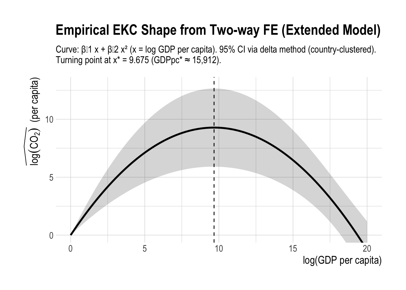
# EKC shape + 95% band (country-clustered), plotted over x in [0, 20], y in [0, 13]# 0) Cluster-robust vcovV <-vcovHC(m3_twfe_ext, type ="HC1", cluster ="group")# 1) Coefs (GDP terms only)b <-coef(m3_twfe_ext)b1 <-unname(b["log_gdppc"])b2 <-unname(b["log_gdppc2"])# 2) Grid over requested rangeekc_shape_df <-tibble(x =seq(0, 20, length.out =400)) |>mutate(ekc_shape = b1 * x + b2 * x^2)# 3) Delta-method SE for m(x) = b1*x + b2*x^2V_sub <- V[c("log_gdppc", "log_gdppc2"), c("log_gdppc", "log_gdppc2")]ekc_shape_df <- ekc_shape_df |>rowwise() |>mutate(se =sqrt(c(x, x^2) %*% V_sub %*%c(x, x^2)),lo = ekc_shape -1.96* se,hi = ekc_shape +1.96* se ) |>ungroup()# 4) Turning pointx_star <--b1 / (2* b2)gdppc_star <-exp(x_star)# 5) Plotggplot(ekc_shape_df, aes(x = x, y = ekc_shape)) +geom_ribbon(aes(ymin = lo, ymax = hi), alpha =0.2) +geom_line(linewidth =1.1) +geom_vline(xintercept = x_star, linetype ="dashed") +coord_cartesian(xlim =c(0, 20), ylim =c(0, 13)) +labs(title ="Empirical EKC Shape from Two-way FE (Extended Model)",subtitle =paste0("Curve: β̂1 x + β̂2 x² (x = log GDP per capita). ","95% CI via delta method (country-clustered). ","\nTurning point at x* = ", round(x_star, 3)," (GDPpc* ≈ ", scales::comma(round(gdppc_star, 0)), ")." ),x ="log(GDP per capita)",y =expression(widehat(log(CO[2]))~~"(per capita)") )