Lasso Linear Regression

Online Shopping

from google.colab import data_table
data_table.enable_dataframe_formatter()  # Enabling an interactive DataFrame display

import numpy as np
import pandas as pd
import matplotlib.pyplot as plt
import seaborn as sns

from sklearn.preprocessing import scale # zero mean & one s.d.
from sklearn.linear_model import LassoCV, lasso_path
from sklearn.model_selection import train_test_split
from sklearn.metrics import mean_squared_error

df = pd.read_csv("https://bcdanl.github.io/data/browser-online-shopping.zip")
df

Warning: Total number of columns (1001) exceeds max_columns (20). Falling back to pandas display.

	spend	atdmt.com	yahoo.com	whenu.com	weatherbug.com	msn.com	google.com	aol.com	questionmarket.com	googlesyndication.com-o02	...	ugo.com	cox.com	spicymint.com	real.com-o01	targetnet.com	effectivebrand.com	dallascowboys.com	leadgenetwork.com	in.us	vistaprint.com
0	424	4.052026	11.855928	0.000000	0.000000	0.250125	6.528264	0.150075	1.350675	3.401701	...	0.0	0.025013	0.000000	0.000000	0.000000	0.0	0.0	0.0	0.0	0.000000
1	2335	4.448743	8.446164	0.000000	0.000000	0.644745	0.451322	0.128949	0.967118	1.225016	...	0.0	0.000000	0.000000	0.000000	0.000000	0.0	0.0	0.0	0.0	0.000000
2	279	7.678815	0.487234	0.000000	31.904112	13.213798	0.954980	0.000000	2.124342	2.514130	...	0.0	0.000000	0.000000	0.019489	0.019489	0.0	0.0	0.0	0.0	0.000000
3	829	13.547802	18.509289	0.045310	0.045310	0.294517	1.110104	0.067966	3.194382	3.149071	...	0.0	0.000000	0.000000	0.000000	0.000000	0.0	0.0	0.0	0.0	0.067966
4	221	2.879581	10.558464	0.000000	0.000000	3.606748	1.396161	0.000000	0.727167	0.988947	...	0.0	0.000000	0.000000	0.000000	0.000000	0.0	0.0	0.0	0.0	0.000000
...	...	...	...	...	...	...	...	...	...	...	...	...	...	...	...	...	...	...	...	...	...
9995	102	6.040454	26.350790	0.000000	0.000000	0.000000	0.055417	4.710446	2.909393	0.554170	...	0.0	0.000000	0.000000	0.000000	0.000000	0.0	0.0	0.0	0.0	0.000000
9996	5096	8.044292	3.012539	9.102752	0.032568	1.612115	1.840091	9.037616	3.289367	1.009608	...	0.0	0.000000	0.000000	0.000000	0.000000	0.0	0.0	0.0	0.0	0.000000
9997	883	7.053942	1.659751	0.000000	0.000000	9.543568	0.414938	13.692946	2.074689	2.074689	...	0.0	0.000000	0.000000	0.000000	0.000000	0.0	0.0	0.0	0.0	0.000000
9998	256	10.408043	0.473093	0.000000	0.000000	18.568894	0.887049	3.370787	3.548196	0.236546	...	0.0	0.532229	0.000000	0.000000	0.000000	0.0	0.0	0.0	0.0	0.000000
9999	6	2.937832	11.789234	0.018954	7.827900	0.113723	2.710387	0.151630	0.777104	0.398029	...	0.0	0.000000	0.037908	0.000000	0.000000	0.0	0.0	0.0	0.0	0.000000

10000 rows × 1001 columns

X = df.drop('spend', axis = 1)
y = df['spend']

# Train-test split
X_train, X_test, y_train, y_test = train_test_split(X, y, test_size=0.2, random_state=42)


X_train_np = X_train.values
X_test_np = X_test.values
y_train_np = y_train.values
y_test_np = y_test.values

# LassoCV with a range of alpha values
lasso_cv = LassoCV(n_alphas = 100, # default is 100
                   alphas = None, # alphas=None automatically generate 100 candidate alpha values
                   cv = 5,
                   random_state=42,
                   max_iter=100000)
lasso_cv.fit(X_train.values, np.log(y_train.values))

print("LassoCV - Best alpha:", lasso_cv.alpha_)


# Create a DataFrame including the intercept and the coefficients:
coef_lasso = pd.DataFrame({
    'predictor': list(X_train.columns),
    'coefficient':  list(lasso_cv.coef_),
    'exp_coefficient': np.exp(  list(lasso_cv.coef_) )
})


# Evaluate
y_pred_lasso = lasso_cv.predict(X_test.values)
mse_lasso = mean_squared_error(y_test, y_pred_lasso)
print("LassoCV - MSE:", mse_lasso)

LassoCV - Best alpha: 0.004098154620620373
LassoCV - MSE: 88099012.81854005

# LassoCV with a range of alpha values
lasso_cv = LassoCV(n_alphas = 100, # default is 100
                   alphas = None, # alphas=None automatically generate 100 candidate alpha values
                   cv = 5,
                   random_state=42,
                   max_iter=100000)
lasso_cv.fit(X_train_np, np.log(y_train_np))

print("LassoCV - Best alpha:", lasso_cv.alpha_)


# Create a DataFrame including the intercept and the coefficients:
coef_lasso = pd.DataFrame({
    'predictor': list(X_train.columns),
    'coefficient':  list(lasso_cv.coef_),
    'exp_coefficient': np.exp(  list(lasso_cv.coef_) )
})


# Evaluate
y_pred_lasso = lasso_cv.predict(X_test_np)
mse_lasso = mean_squared_error(y_test_np, y_pred_lasso)
print("LassoCV - MSE:", mse_lasso)

LassoCV - Best alpha: 0.004098154620620373
LassoCV - MSE: 88099012.81854005

coef_lasso = coef_lasso.query('coefficient != 0')
coef_lasso.shape[0]

307

coef_lasso.sort_values('coefficient', ascending = False)

	predictor	coefficient	exp_coefficient
895	bizrate.com-o01	1.388699	4.009628
770	staples.com	0.757120	2.132127
690	travelhook.net	0.688146	1.990022
843	united.com	0.610771	1.841850
506	victoriassecret.com	0.584030	1.793251
...	...	...	...
279	new.net	-0.181475	0.834039
374	coolsavings.com	-0.187875	0.828718
851	rsc03.net	-0.231599	0.793264
443	checkm8.com	-0.240327	0.786371
481	macromedia.com	-0.243739	0.783693

307 rows × 3 columns

# Compute the mean and standard deviation of the CV errors for each alpha.
mean_cv_errors = np.mean(lasso_cv.mse_path_, axis=1)
std_cv_errors = np.std(lasso_cv.mse_path_, axis=1)

plt.figure(figsize=(8, 6))
plt.errorbar(lasso_cv.alphas_, mean_cv_errors, yerr=std_cv_errors, marker='o', linestyle='-', capsize=5)
plt.xscale('log')
plt.xlabel('Alpha')
plt.ylabel('Mean CV Error (MSE)')
plt.title('Cross-Validation Error vs. Alpha')
#plt.gca().invert_xaxis()  # Optionally invert the x-axis so lower alphas (less regularization) appear to the right.
plt.axvline(x=lasso_cv.alpha_, color='red', linestyle='--', label='Best alpha')
plt.legend()
plt.show()

# Compute the coefficient path over the alpha grid that LassoCV used
alphas, coefs, _ = lasso_path(X_train, np.log(y_train),
                              alphas=lasso_cv.alphas_,
                              max_iter=100000)

# Count nonzero coefficients for each alpha (coefs shape: (n_features, n_alphas))
nonzero_counts = np.sum(coefs != 0, axis=0)

# Plot the number of nonzero coefficients versus alpha
plt.figure(figsize=(8,6))
plt.plot(alphas, nonzero_counts, marker='o', linestyle='-')
plt.xscale('log')
plt.xlabel('Alpha')
plt.ylabel('Number of nonzero coefficients')
plt.title('Nonzero Coefficients vs. Alpha')
#plt.gca().invert_xaxis()  # Lower alphas (less regularization) on the right
plt.axvline(x=lasso_cv.alpha_, color='red', linestyle='--', label='Best alpha')
plt.legend()
plt.show()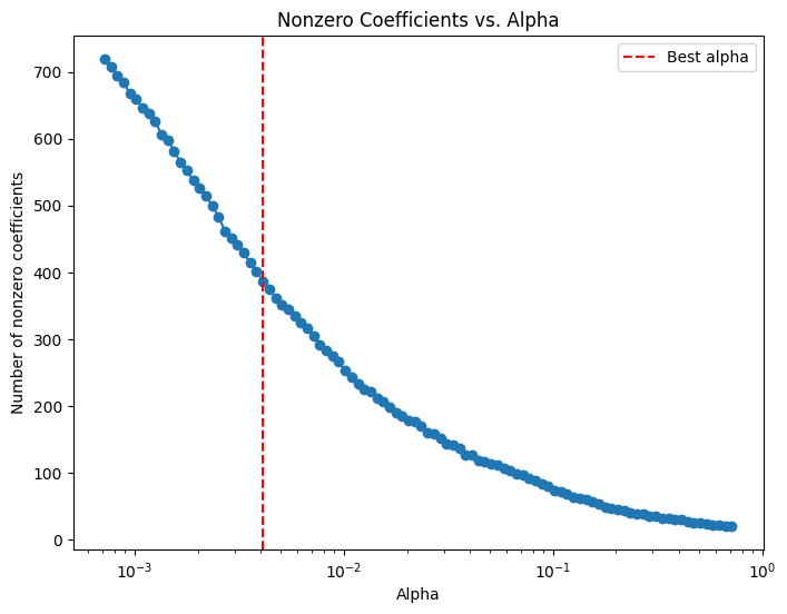

# Compute the lasso path. Note: we use np.log(y_train) because that's what you used in LassoCV.
alphas, coefs, _ = lasso_path(X_train.values, np.log(y_train.values), alphas=lasso_cv.alphas_, max_iter=100000)

plt.figure(figsize=(8, 6))
# Iterate over each predictor and plot its coefficient path.
for i, col in enumerate(X_train.columns):
    plt.plot(alphas, coefs[i, :], label=col)

plt.xscale('log')
plt.xlabel('Alpha')
plt.ylabel('Coefficient value')
plt.title('Lasso Coefficient Paths')
#plt.gca().invert_xaxis()  # Lower alphas (weaker regularization) to the right.
#plt.legend(bbox_to_anchor=(1.05, 1), loc='upper left')
plt.axvline(x=lasso_cv.alpha_, color='red', linestyle='--', label='Best alpha')
#plt.legend()
plt.show()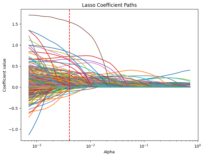

# RidgeCV with a list of alpha values and 3-fold cross-validation
from sklearn.linear_model import RidgeCV, Ridge

alpha_max = 10
alpha_min_ratio = 1e-4
alpha_min = alpha_max * alpha_min_ratio

# Define candidate alpha values
alphas = np.logspace(np.log(alpha_max), np.log(alpha_min), num=5)
alphas

array([2.00717432e+02, 1.00000000e+00, 4.98212830e-03, 2.48216024e-05,
       1.23664407e-07])

ridge_cv = RidgeCV(alphas=alphas, cv=3, scoring='neg_mean_squared_error')
ridge_cv.fit(X_train_np, np.log(y_train_np))

print("RidgeCV - Best alpha:", ridge_cv.alpha_)

# Create a DataFrame including the intercept and the coefficients:
coef_ridge = pd.DataFrame({
    'predictor': list(X_train.columns),
    'coefficient': list(ridge_cv.coef_),
    'exp_coefficient': np.exp( list(ridge_cv.coef_) )
})

# Evaluate
y_pred_ridge = ridge_cv.predict(X_test_np)
mse_ridge = mean_squared_error(y_test_np, y_pred_ridge)
print("RidgeCV - MSE:", mse_ridge)

RidgeCV - Best alpha: 200.71743249053017
RidgeCV - MSE: 88099136.93994579

coef_ridge

	predictor	coefficient	exp_coefficient
0	atdmt.com	-0.004977	0.995035
1	yahoo.com	-0.017194	0.982953
2	whenu.com	-0.008336	0.991699
3	weatherbug.com	-0.005399	0.994616
4	msn.com	-0.004900	0.995112
...	...	...	...
995	effectivebrand.com	-0.098469	0.906223
996	dallascowboys.com	-0.039989	0.960800
997	leadgenetwork.com	0.009274	1.009317
998	in.us	-0.033527	0.967029
999	vistaprint.com	0.066156	1.068394

1000 rows × 3 columns

coef_ridge.query('coefficient != 0').shape[0]

1000

ridge = Ridge()
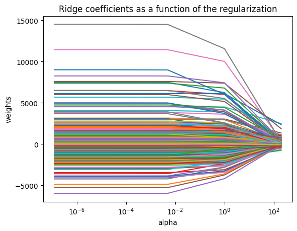
coefs = []

for a in alphas:
    ridge.set_params(alpha=a)
    ridge.fit(X_train_np, y_train_np)
    coefs.append(ridge.coef_)

ax = plt.gca()
ax.plot(alphas, coefs)
ax.set_xscale('log')
#ax.set_xlim(ax.get_xlim()[::-1])  # reverse axis
plt.axis('tight')
plt.xlabel('alpha')
plt.ylabel('weights')
plt.title('Ridge coefficients as a function of the regularization');