Random Forest and Gradient-Boosted Trees

Boston Housing Data

Author

Byeong-Hak Choe

Published

March 30, 2026

Modified

April 13, 2026

library(tidyverse)
library(janitor)
library(ggthemes)
library(rmarkdown)

library(rpart)
library(rpart.plot)
library(ranger)
library(vip)
library(pdp)
# library(xgboost) # load this right before we use xgboost()

Boston Housing Data

boston <- read_csv("https://bcdanl.github.io/data/boston.csv") |>
  janitor::clean_names()

paged_table(boston)

Modeling goal

Predict medv, median housing value in thousands of dollars
Boston housing is a classic regression example with multiple socioeconomic and neighborhood predictors
We will use it to study overfitting, pruning, random forests, and boosting

Create training and test data

set.seed(42120532)
boston <- boston |> 
  mutate(rnd = runif(n()))

dtrain <- boston |> 
  filter(rnd > .2) |> 
  select(-rnd)

dtest <- boston |> 
  filter(rnd <= .2) |> 
  select(-rnd)

x_train <- dtrain |> select(-medv)
y_train <- dtrain$medv
x_test  <- dtest |> select(-medv)
y_test  <- dtest$medv

Random Forest

Fit an initial random forest on Boston housing

set.seed(1917)

init_boston_rf <- ranger(
  medv ~ .,
  data = dtrain,
  num.trees = 300,
  importance = "permutation"
)

init_boston_rf

Ranger result

Call:
 ranger(medv ~ ., data = dtrain, num.trees = 300, importance = "permutation") 

Type:                             Regression 
Number of trees:                  300 
Sample size:                      392 
Number of independent variables:  13 
Mtry:                             3 
Target node size:                 5 
Variable importance mode:         permutation 
Splitrule:                        variance 
OOB prediction error (MSE):       11.83664 
R squared (OOB):                  0.8582419

Important `ranger()` arguments

init_boston_rf$num.trees

[1] 300

init_boston_rf$mtry

[1] 3

init_boston_rf$prediction.error

[1] 11.83664

init_boston_rf$min.node.size

[1] 5

init_boston_rf$importance

[1] "permutation"

num.trees: number of trees in the forest
mtry: number of predictors considered at each split
prediction.error: out-of-bag error estimate.
min.node.size: minimum terminal node size
importance: method used to calculate variable importance
- "none": do not compute variable importance (default)
- "impurity": compute importance based on total impurity reduction from splits
- "permutation": compute importance based on how much model performance worsens when a variable is shuffled

Interpreting the `ranger` output

Tune `mtry`

No loop

rf_2 <- ranger(
  medv ~ .,
  data = dtrain,
  num.trees = 300,
  mtry = 2,
  importance = "permutation"
)

rf_4 <- ranger(
  medv ~ .,
  data = dtrain,
  num.trees = 300,
  mtry = 4,
  importance = "permutation"
)

rf_6 <- ranger(
  medv ~ .,
  data = dtrain,
  num.trees = 300,
  mtry = 6,
  importance = "permutation"
)

rf_8 <- ranger(
  medv ~ .,
  data = dtrain,
  num.trees = 300,
  mtry = 8,
  importance = "permutation"
)

rf_10 <- ranger(
  medv ~ .,
  data = dtrain,
  num.trees = 300,
  mtry = 10,
  importance = "permutation"
)

rf_12 <- ranger(
  medv ~ .,
  data = dtrain,
  num.trees = 300,
  mtry = 12,
  importance = "permutation"
)

rf_results <- tibble(
  mtry = c(2, 4, 6, 8, 10, 12),
  oob_error = c(
    rf_2$prediction.error,
    rf_4$prediction.error,
    rf_6$prediction.error,
    rf_8$prediction.error,
    rf_10$prediction.error,
    rf_12$prediction.error
  )
)

rf_results |>
  paged_table()

Loop

# p = the total number of predictor variables in the training data
p <- ncol(x_train)

# Create a tuning grid for mtry:
# mtry is the number of predictors randomly considered at each split
# Here, we try even-numbered values from 2 up to p
rf_grid <- tibble(mtry = seq(2, p, by = 2))

# Create an empty tibble to store the tuning results
# We will save each mtry value and its corresponding OOB error
rf_results <- tibble(
  mtry = numeric(),
  oob_error = numeric()
)

# Loop over each candidate mtry value
for (m in rf_grid$mtry) {
  
  # Fit a random forest model with the current mtry value
  fit <- ranger(
    medv ~ .,                 
    data = dtrain,            
    num.trees = 300,          # grow 300 trees in the forest
    mtry = m,                 # current candidate value of mtry
    importance = "permutation" # compute permutation-based variable importance
  )

  # Store the current mtry value and its OOB prediction error
  rf_results <- bind_rows(
    rf_results,
    tibble(
      mtry = m,
      oob_error = fit$prediction.error
    )
  )
}


rf_results |> 
  paged_table()

Plot the tuning results

rf_results |>
  ggplot(aes(x = mtry, y = oob_error)) +
  geom_line() +
  geom_point() +
  labs(
    title = "Random Forest Tuning Results",
    x = "mtry",
    y = "Out-of-bag prediction error"
  )

Final random forest

best_mtry <- rf_results |>
  slice_min(oob_error, n = 1) |>
  pull(mtry)

final_boston_rf <- ranger(
  medv ~ .,
  data = dtrain,
  num.trees = 500,
  mtry = best_mtry,
  importance = "permutation"
)

best_mtry

[1] 10

final_boston_rf

Ranger result

Call:
 ranger(medv ~ ., data = dtrain, num.trees = 500, mtry = best_mtry,      importance = "permutation") 

Type:                             Regression 
Number of trees:                  500 
Sample size:                      392 
Number of independent variables:  13 
Mtry:                             10 
Target node size:                 5 
Variable importance mode:         permutation 
Splitrule:                        variance 
OOB prediction error (MSE):       9.527965 
R squared (OOB):                  0.8858911

Test performance of the random forest

rf_test_pred <- predict(final_boston_rf, data = dtest)$predictions

sqrt(mean((y_test - rf_test_pred)^2))

[1] 3.075023

Random forest variable importance

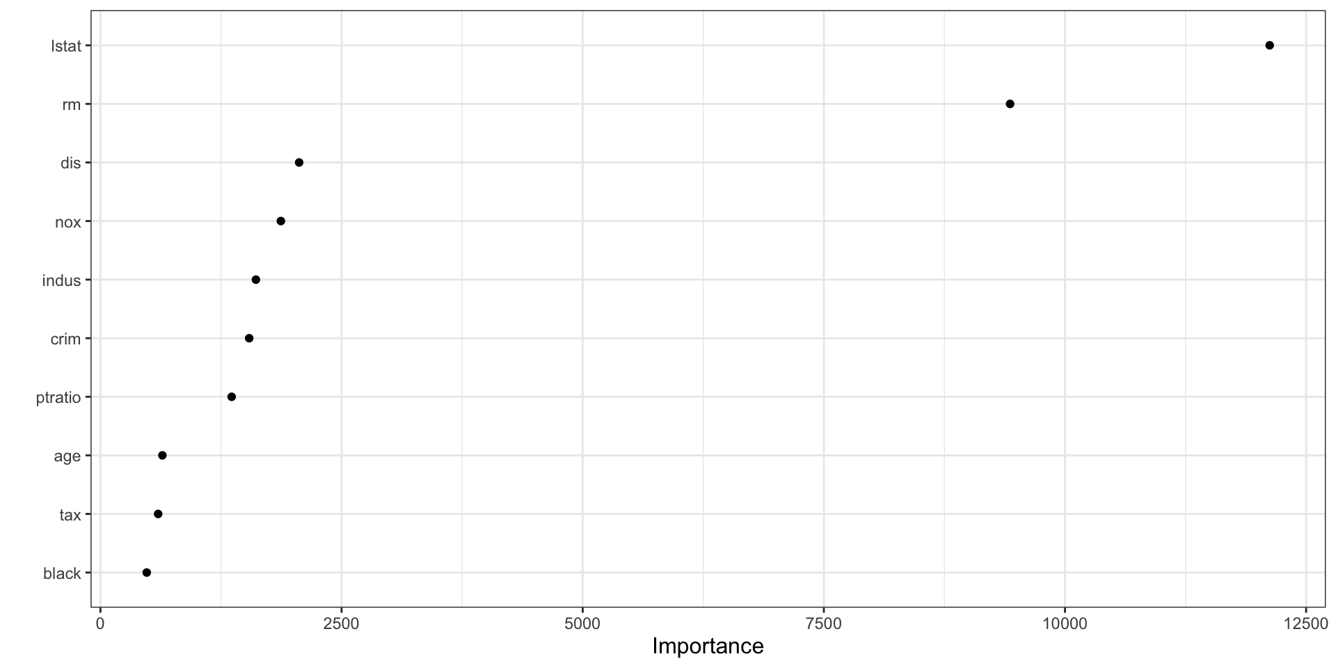
vip(final_boston_rf)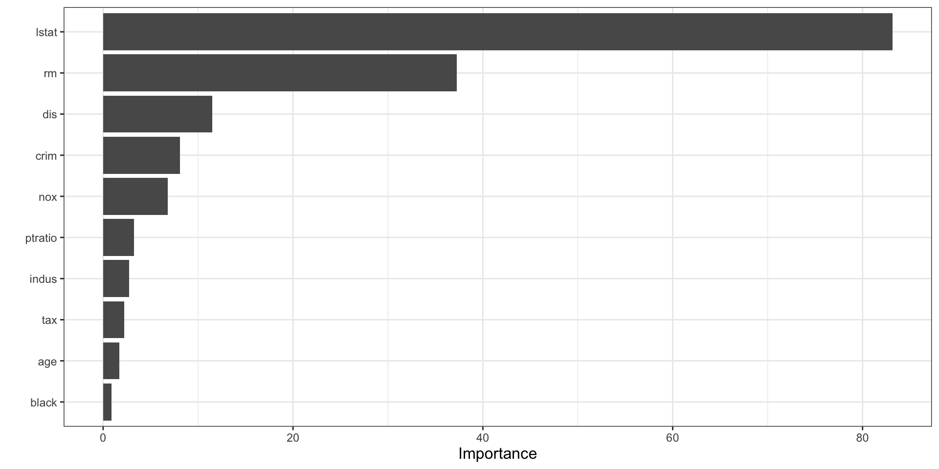

How to interpret `vip()` for a random forest

The plot shows which predictors contributed most across the ensemble of trees.
Higher importance means a variable was more useful in improving splits across the forest.
In forests, importance is often more stable than in a single tree because it aggregates over many trees.

Partial dependence from the forest

partial(final_boston_rf, pred.var = "lstat", train = x_train) |>
  autoplot() +
  labs(title = "Partial Dependence of MEDV on LSTAT")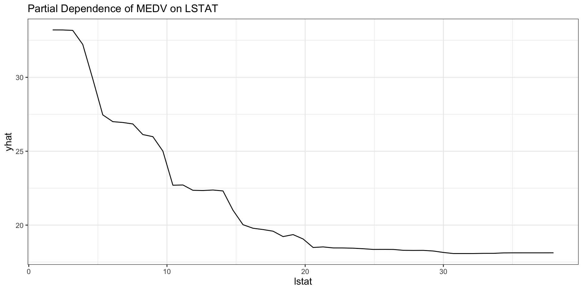

Interpreting the random-forest PDP

The curve shows the model’s average predicted medv as lstat changes.
All other variables are averaged over their observed values.
Nonlinearity in the curve suggests that the marginal relationship is not well described by a straight line.
Flat regions suggest limited marginal predictive contribution in that range.

Gradient-Boosted Trees

Key XGBoost tuning arguments

nrounds: number of boosting iterations
eta: learning rate
max_depth: depth of each tree
gamma: minimum improvement required for a split
subsample: fraction of observations used for each boosting step
colsample_bytree: fraction of predictors used for each tree
min_child_weight: minimum total weight allowed in a child node

How to think about the main tuning parameters

Smaller eta means slower learning and usually requires larger nrounds.
Larger max_depth allows more complex interactions.
Larger gamma makes splitting more conservative.
Smaller subsample and colsample_bytree can reduce overfitting by injecting randomness.
nrounds and eta usually need to be tuned together.

Prepare matrix input for XGBoost

x_train_mat <- as.matrix(x_train)
x_test_mat  <- as.matrix(x_test)

Fit an initial XGBoost model

library(xgboost)

set.seed(1937)

xgb_fit_initial <- xgboost(
  data = x_train_mat,
  label = y_train,
  objective = "reg:squarederror",
  nrounds = 100,
  eta = 0.1,
  max_depth = 3,
  verbose = 0
)

xgb_fit_initial

XGBoost model object
Call:
  xgboost(objective = "reg:squarederror", nrounds = 100, max_depth = 3, 
    data = x_train_mat, label = y_train, eta = 0.1, verbose = 0)
Objective: reg:squarederror
Number of iterations: 100
Number of features: 13

What does the initial model represent?

It is a sum of many shallow trees, not one large tree.
Each boosting round adds a small correction to the current prediction.

`objective` in `xgboost()`

objective = "reg:squarederror" is used for a regression problem, where the response variable is continuous.
- It tells XGBoost to predict a numeric outcome and minimize squared prediction error.
objective = "binary:logistic" is used for a binary classification problem, where the response variable has two classes such as 0 and 1.
- It tells XGBoost to predict the probability that an observation belongs to class 1.

Simple tuning grid

xgb_grid <- tidyr::crossing(
  nrounds = seq(50, 250, by = 50),
  eta = c(0.025, 0.05, 0.1),
  max_depth = c(1, 2, 3, 4),
  gamma = c(0, 1),
  colsample_bytree = c(0.8, 1),
  min_child_weight = 1,
  subsample = c(0.8, 1)
)

xgb_grid |> 
  paged_table()

tidyr::crossing() generates all possible combinations of the supplied values, which is exactly what you want for a manual grid search.

Grid size: 5 × 3 × 4 × 2 × 2 × 1 × 2 = 480 combinations
min_child_weight = 1 is held constant (scalar), while everything else is varied
Here, nrounds and eta are treated independently — combinations like nrounds = 50, eta = 0.025 (very slow learning, few rounds) will both be evaluated alongside nrounds = 250, eta = 0.1
- We can consider fixing eta and using early stopping instead, which makes nrounds a ceiling rather than a tuning parameter

Cross-validated tuning

xgb_results_lst <- vector("list", nrow(xgb_grid))

dMat_train <- xgb.DMatrix(data = x_train_mat, label = y_train)

for (i in seq_len(nrow(xgb_grid))) {
  nrounds <- xgb_grid$nrounds[i]
  eta <- xgb_grid$eta[i]
  max_depth <- xgb_grid$max_depth[i]
  gamma <- xgb_grid$gamma[i]
  colsample_bytree <- xgb_grid$colsample_bytree[i]
  min_child_weight <- xgb_grid$min_child_weight[i]
  subsample <- xgb_grid$subsample[i]

  cv_fit <- xgb.cv(
    # data = x_train_mat,
    # label = y_train,
    
    # If an error occurs with the message including DMatrix, try:
    data = dMat_train,
  
    nrounds = nrounds,
    nfold = 5,
    objective = "reg:squarederror",
    eta = eta,
    max_depth = max_depth,
    gamma = gamma,
    colsample_bytree = colsample_bytree,
    min_child_weight = min_child_weight,
    subsample = subsample,
    verbose = 0
  )

  xgb_results_lst[[i]] <- tibble(
    nrounds = nrounds,
    eta = eta,
    max_depth = max_depth,
    gamma = gamma,
    colsample_bytree = colsample_bytree,
    min_child_weight = min_child_weight,
    subsample = subsample,
    cv_rmse = min(cv_fit$evaluation_log$test_rmse_mean)
  )
}

xgb_results <- 
  bind_rows(xgb_results_lst) |> 
  arrange(cv_rmse)

xgb_results |> 
  paged_table()

Fit the final XGBoost model

# best_xgb <- xgb_results[order(xgb_results$cv_rmse), ][1, ]

best_xgb <- xgb_results |>
  slice_min(cv_rmse, n = 1)

best_xgb |> 
  paged_table()

xgb_fit_final <- xgboost(
  data = x_train_mat,
  label = y_train,
  objective = "reg:squarederror",
  nrounds = best_xgb$nrounds,
  eta = best_xgb$eta,
  max_depth = best_xgb$max_depth,
  gamma = best_xgb$gamma,
  colsample_bytree = best_xgb$colsample_bytree,
  min_child_weight = best_xgb$min_child_weight,
  subsample = best_xgb$subsample,
  verbose = 0
)

xgb_fit_final

XGBoost model object
Call:
  xgboost(objective = "reg:squarederror", nrounds = best_xgb$nrounds, 
    max_depth = best_xgb$max_depth, min_child_weight = best_xgb$min_child_weight, 
    subsample = best_xgb$subsample, colsample_bytree = best_xgb$colsample_bytree, 
    data = x_train_mat, label = y_train, eta = best_xgb$eta, 
    gamma = best_xgb$gamma, verbose = 0)
Objective: reg:squarederror
Number of iterations: 150
Number of features: 13

Test performance of XGBoost

xgb_test_pred <- predict(xgb_fit_final, newdata = x_test_mat)

sqrt(mean((y_test - xgb_test_pred)^2))

[1] 2.841075

Variable Importance: A Free Byproduct of Ensembles

Both random forest and gradient boosting measure variable importance automatically
The key question: how much does each predictor contribute to reducing prediction error?
Random forest — permutation importance:
- For each variable, randomly shuffle its values and measure the drop in OOB accuracy
- A large drop → the variable was doing real work; a small drop → it barely mattered
Random forest — impurity importance:
- Tracks how much splits on a variable reduce impurity, summed across all trees
- In regression, impurity is usually based on reduction in outcome variance
- A larger total reduction means the variable was more useful for making cleaner splits
Gradient boosting — gain-based importance:
- Tracks how much each split on a variable reduced the loss function, summed across all trees
- Variables used in high-gain splits rank highly

Why This Matters

Unlike linear regression, tree ensembles can capture non-linear effects and interactions. Variable importance tells you which variables the model relies on most, even when the relationship between predictor and outcome is complex.

XGBoost variable importance

vip(xgb_fit_final) +
  labs(title = "XGBoost Variable Importance")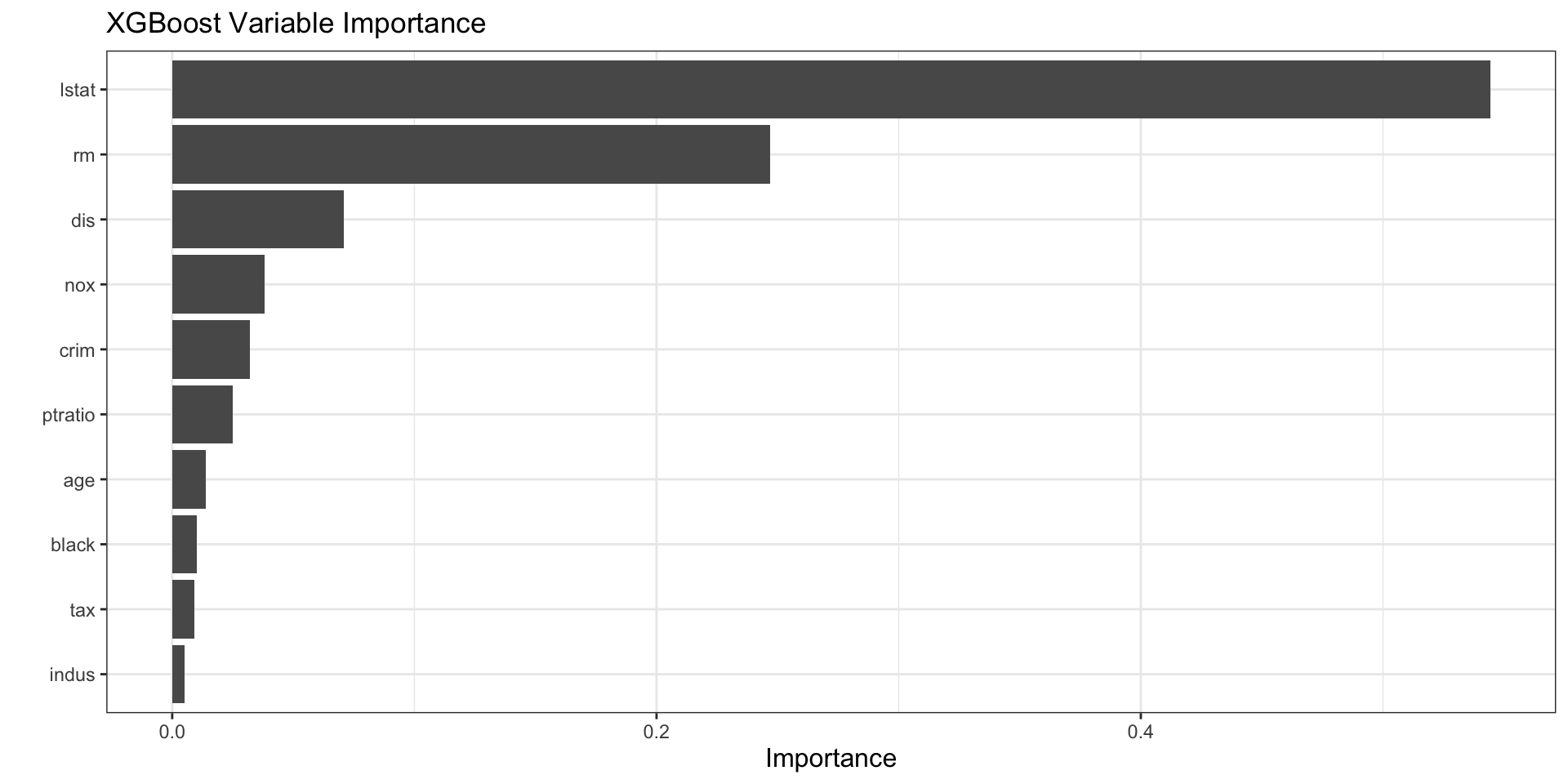

How to interpret `vip()` for XGBoost

XGBoost importance is based on how much each variable contributes across many boosting rounds.
Variables near the top are most useful for reducing the loss function.
Importance does not reveal the direction of the effect.
A variable can be important because it appears in many small improvements, not only because it appears in one dominant split.

Partial dependence for XGBoost

partial(
  xgb_fit_final,
  pred.var = "lstat",
  train = x_train_mat,
  plot = TRUE,
  plot.engine = "ggplot2",
  type = "regression"
) +
  labs(title = "Partial Dependence of MEDV on LSTAT")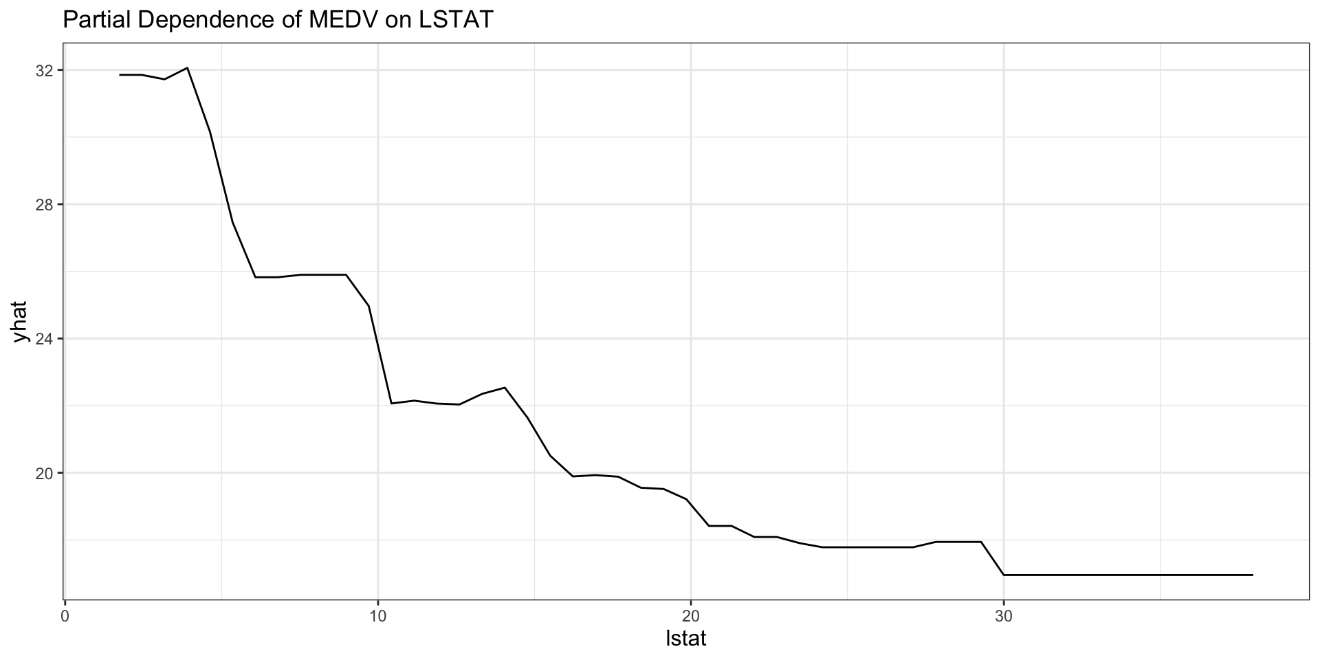

Interpreting the XGBoost PDP

The PDP summarizes the average fitted relationship between lstat and predicted housing values.
Because XGBoost is highly flexible, the curve can show richer nonlinearities than a single tree.
Sharp changes in the curve can indicate thresholds learned by the boosted ensemble.

Boston Housing Data

Modeling goal

Create training and test data

Random Forest

Fit an initial random forest on Boston housing

Important ranger() arguments

Interpreting the ranger output

Tune mtry

No loop

Loop

Plot the tuning results

Final random forest

Test performance of the random forest

Random forest variable importance

How to interpret vip() for a random forest

Partial dependence from the forest

Interpreting the random-forest PDP

Gradient-Boosted Trees

Key XGBoost tuning arguments

How to think about the main tuning parameters

Prepare matrix input for XGBoost

Fit an initial XGBoost model

What does the initial model represent?

objective in xgboost()

Simple tuning grid

Cross-validated tuning

Fit the final XGBoost model

Test performance of XGBoost

Variable Importance: A Free Byproduct of Ensembles

XGBoost variable importance

How to interpret vip() for XGBoost

Partial dependence for XGBoost

Interpreting the XGBoost PDP

Important `ranger()` arguments

Interpreting the `ranger` output

Tune `mtry`

How to interpret `vip()` for a random forest

`objective` in `xgboost()`

How to interpret `vip()` for XGBoost