library(tidyverse)
library(broom)
library(stargazer)
library(margins)
library(yardstick)
library(WVPlots)
library(pROC)
library(glmnet)
library(gamlr)

library(DT)
library(rmarkdown)
library(hrbrthemes)
library(ggthemes)

theme_set(
  theme_ipsum()
)

scale_colour_discrete <- function(...) scale_color_colorblind(...)
scale_fill_discrete <- function(...) scale_fill_colorblind(...)Regularized Logistic Regression
Car Safety Inspection
R Packages and Settings
Data
df <- read_csv('https://bcdanl.github.io/data/car-data.csv')

df |>
  rmarkdown::paged_table()
Variable description
| Variable | Description |
|---|---|
buying |
Buying price of the car (vhigh, high, med, low) |
maint |
Maintenance cost (vhigh, high, med, low) |
doors |
Number of doors (2, 3, 4, 5more) |
persons |
Capacity in terms of persons to carry (2, 4, more) |
lug_boot |
Size of luggage boot (small, med, big) |
safety |
Estimated safety of the car (low, med, high) |
rating |
Car acceptability (unacc, acc, good, vgood) |
fail |
TRUE if the car is unacceptable (unacc), otherwise FALSE |
Quick check
df |>
  count(buying)
# A tibble: 4 × 2
buying n
<chr> <int>
1 high 432
2 low 432
3 med 432
4 vhigh 432df |>
count(maint)# A tibble: 4 × 2
maint n
<chr> <int>
1 high 432
2 low 432
3 med 432
4 vhigh 432df |>
count(doors)# A tibble: 4 × 2
doors n
<chr> <int>
1 2 432
2 3 432
3 4 432
4 5more 432df |>
count(persons)# A tibble: 3 × 2
persons n
<chr> <int>
1 2 576
2 4 576
3 more 576df |>
count(lug_boot)# A tibble: 3 × 2
lug_boot n
<chr> <int>
1 big 576
2 med 576
3 small 576df |>
count(safety)# A tibble: 3 × 2
safety n
<chr> <int>
1 high 576
2 low 576
3 med 576Model
\[ \begin{align} &\quad\;\; \text{Prob}(\text{fail}_{i} = 1) \\ &= G\Big(\beta_{0} \\ &\qquad\quad\;\;\; \,+\, \beta_{4} \text{buying\_med}_{i} \,+\, \beta_{4} \text{buying\_high}_{i} \,+\, \beta_{4} \text{buying\_vhigh}_{i} \\ &\qquad\quad\;\;\; \,+\, \beta_{4} \text{maint\_med}_{i} \,+\, \beta_{4} \text{maint\_high}_{i} \,+\, \beta_{4} \text{maint\_vhigh}_{i} \\ &\qquad\quad\;\;\; \,+\, \beta_{7} \text{persons\_4}_{i} \,+\, \beta_{8} \text{persons\_more}_{i} \\ &\qquad\quad\;\;\; \,+\, \beta_{10} \text{lug\_boot\_med}_{i}\,+\, \beta_{10} \text{lug\_boot\_big}_{i} \\ &\qquad\quad\;\;\; \,+\, \beta_{11} \text{safety\_med}_{i}\,+\, \beta_{11} \text{safety\_high}_{i} \Big), \end{align} \]
where \(G(\,\cdot\,)\) is
\[ G(\,\cdot\,) = \frac{\exp(\,\cdot\,)}{1 + \exp(\,\cdot\,)}. \]
Pre-process & Train/Test Split (runif(n()))
This avoids predict() errors like “factor has new levels …”.
set.seed(14454)
df <- df |>
  mutate(rnd = runif(n())) |>
  mutate(buying = factor(buying),
         buying = fct_relevel(buying, "low"),
         maint = factor(maint),
         maint = fct_relevel(maint, "low"),
         persons = factor(persons),
         persons = fct_relevel(persons, "2"),
         lug_boot = factor(lug_boot),
         lug_boot = fct_relevel(lug_boot, "small"),
         safety = factor(safety),
         safety = fct_relevel(safety, "low"))

dtrain <- df |>
  filter(rnd > .3)
dtest <- df |>
  filter(rnd <= .3)
Logistic Regression
Fit with glm( family = binomial(link = "logit") )
fmla <- fail ~ buying + maint + persons + lug_boot + safety

model <- glm(
  fmla,
  data = dtrain,
  family = binomial(link = "logit")
)
Regression Table (stargazer)
stargazer(
  model,
  type = "html",
  digits = 3,
  title = "Logistic regression (logit): Car Safety"
)| Dependent variable: | |
| fail | |
| buyinghigh | 4.606*** |
| (0.606) | |
| buyingmed | 0.680 |
| (0.548) | |
| buyingvhigh | 6.151*** |
| (0.696) | |
| mainthigh | 3.220*** |
| (0.526) | |
| maintmed | 0.343 |
| (0.487) | |
| maintvhigh | 5.685*** |
| (0.666) | |
| persons4 | -27.530 |
| (948.137) | |
| personsmore | -27.177 |
| (948.137) | |
| lug_bootbig | -3.684*** |
| (0.476) | |
| lug_bootmed | -2.415*** |
| (0.415) | |
| safetyhigh | -28.026 |
| (959.275) | |
| safetymed | -25.413 |
| (959.275) | |
| Constant | 48.862 |
| (1,348.767) | |
| Observations | 1,231 |
| Log Likelihood | -139.963 |
| Akaike Inf. Crit. | 305.926 |
| Note: | p<0.1; p<0.05; p<0.01 |
- Regression table with
summary()
summary(model)
Call:
glm(formula = fmla, family = binomial(link = "logit"), data = dtrain)

Coefficients:
             Estimate Std. Error z value Pr(>|z|)
(Intercept)   48.8619  1348.7670   0.036    0.971
buyinghigh     4.6064     0.6058   7.604 2.88e-14 ***
buyingmed      0.6797     0.5484   1.239    0.215
buyingvhigh    6.1514     0.6965   8.832  < 2e-16 ***
mainthigh      3.2203     0.5259   6.124 9.15e-10 ***
maintmed       0.3432     0.4867   0.705    0.481
maintvhigh     5.6849     0.6661   8.535  < 2e-16 ***
persons4     -27.5300   948.1374  -0.029    0.977
personsmore  -27.1767   948.1374  -0.029    0.977
lug_bootbig   -3.6837     0.4757  -7.744 9.66e-15 ***
lug_bootmed   -2.4148     0.4155  -5.812 6.17e-09 ***
safetyhigh   -28.0256   959.2748  -0.029    0.977
safetymed    -25.4128   959.2746  -0.026    0.979
---
Signif. codes:  0 '***' 0.001 '**' 0.01 '*' 0.05 '.' 0.1 ' ' 1

(Dispersion parameter for binomial family taken to be 1)

    Null deviance: 1477.11  on 1230  degrees of freedom
Residual deviance:  279.93  on 1218  degrees of freedom
AIC: 305.93

Number of Fisher Scoring iterations: 20
Beta Estimates (tidy())
model_betas <- tidy(model,
conf.int = T) # conf.level = 0.95 (default)
model_betas_90ci <- tidy(model,
conf.int = T,
conf.level = 0.90)
model_betas_99ci <- tidy(model,
conf.int = T,
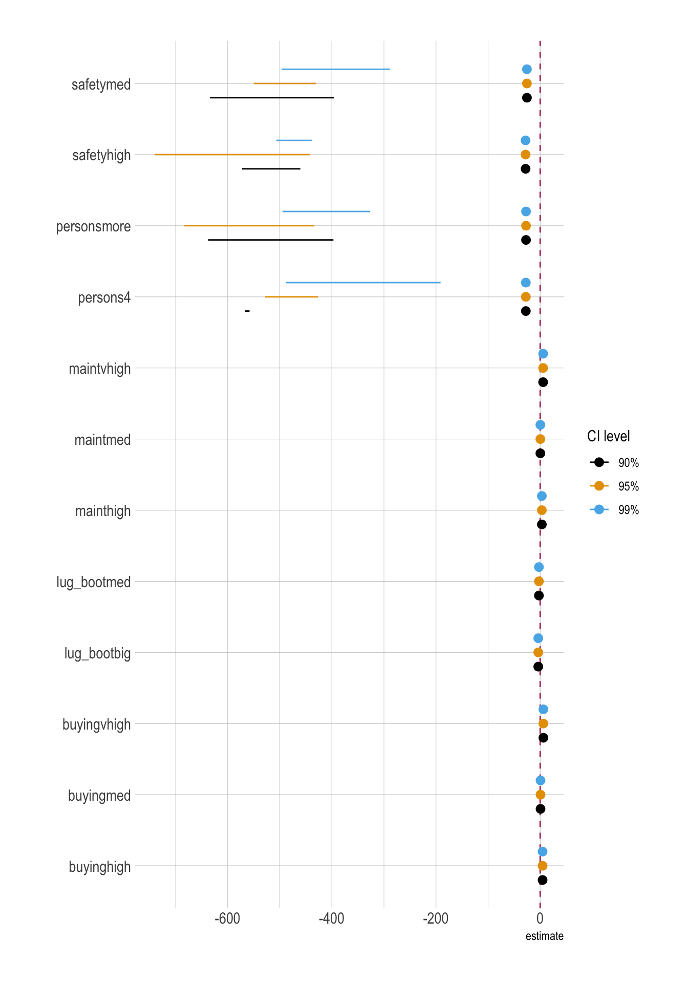
conf.level = 0.99)Coefficient Plots
month_ci <- bind_rows(
  model_betas_90ci |> mutate(ci = "90%"),
  model_betas      |> mutate(ci = "95%"),
  model_betas_99ci |> mutate(ci = "99%")
) |>
  mutate(ci = factor(ci, levels = c("90%", "95%", "99%")))

ggplot(
  data = month_ci |>
    filter(!str_detect(term, "Intercept")),
  aes(
    y = term,
    x = estimate,
    xmin = conf.low,
    xmax = conf.high,
    color = ci
  )
) +
  geom_vline(xintercept = 0, color = "maroon", linetype = 2) +
  geom_pointrange(
    position = position_dodge(width = 0.6)
  ) +
  labs(
    color = "CI level",
    y = ""
) 
Model Fit (glance())
model |>
glance() |>
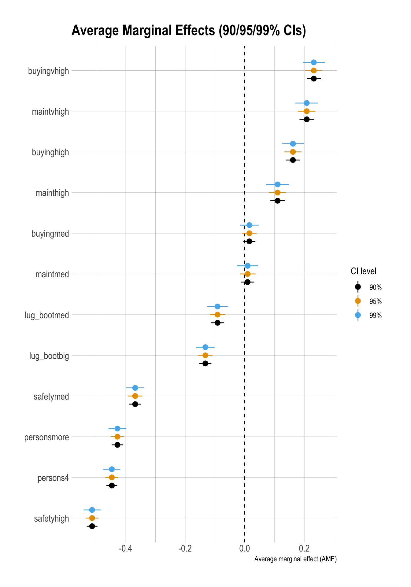
paged_table()Marginal Effects (margins())
Average Marginal Effects
me <- margins(model)
sum_me <- summary(me)
sum_me
factor AME SE z p lower upper
buyinghigh 0.1619 0.0147 11.0250 0.0000 0.1332 0.1907
buyingmed 0.0155 0.0123 1.2599 0.2077 -0.0086 0.0396
buyingvhigh 0.2319 0.0144 16.1105 0.0000 0.2037 0.2601
lug_bootbig -0.1323 0.0123 -10.7690 0.0000 -0.1564 -0.1083
lug_bootmed -0.0915 0.0133 -6.9038 0.0000 -0.1175 -0.0655
mainthigh 0.1103 0.0147 7.4809 0.0000 0.0814 0.1392
maintmed 0.0096 0.0136 0.7097 0.4779 -0.0170 0.0362
maintvhigh 0.2083 0.0148 14.1185 0.0000 0.1793 0.2372
persons4 -0.4467 0.0110 -40.4494 0.0000 -0.4683 -0.4251
personsmore -0.4280 0.0116 -36.8429 0.0000 -0.4508 -0.4052
safetyhigh -0.5130 0.0110 -46.4676 0.0000 -0.5347 -0.4914
safetymed -0.3683 0.0120 -30.5950 0.0000 -0.3919 -0.3447Marginal Effect Plots
df_ame <- sum_me |>
  as_tibble() |>
  rename(
    term = factor,
    ame  = AME,
    se   = SE
  )

# Pair each level with the correct z (NOT a Cartesian product)
ci_levels <- tibble(
  level = c("90%", "95%", "99%"),
  zcrit = c(1.645, 1.96, 2.576)
)

df_ame_ci <- df_ame |>
  tidyr::crossing(level = ci_levels$level) |>
  left_join(ci_levels, by = "level") |>
  mutate(
    conf.low  = ame - zcrit * se,
    conf.high = ame + zcrit * se
  )

ggplot(df_ame_ci,
       aes(x = fct_reorder(term, ame), y = ame)) +
  geom_hline(yintercept = 0, linetype = "dashed") +
  geom_pointrange(
    aes(ymin = conf.low, ymax = conf.high, color = level),
    position = position_dodge(width = 0.6)
  ) +
  coord_flip() +
  labs(
    x = NULL,
    y = "Average marginal effect (AME)",
    color = "CI level",
    title = "Average Marginal Effects (90/95/99% CIs)"
  )
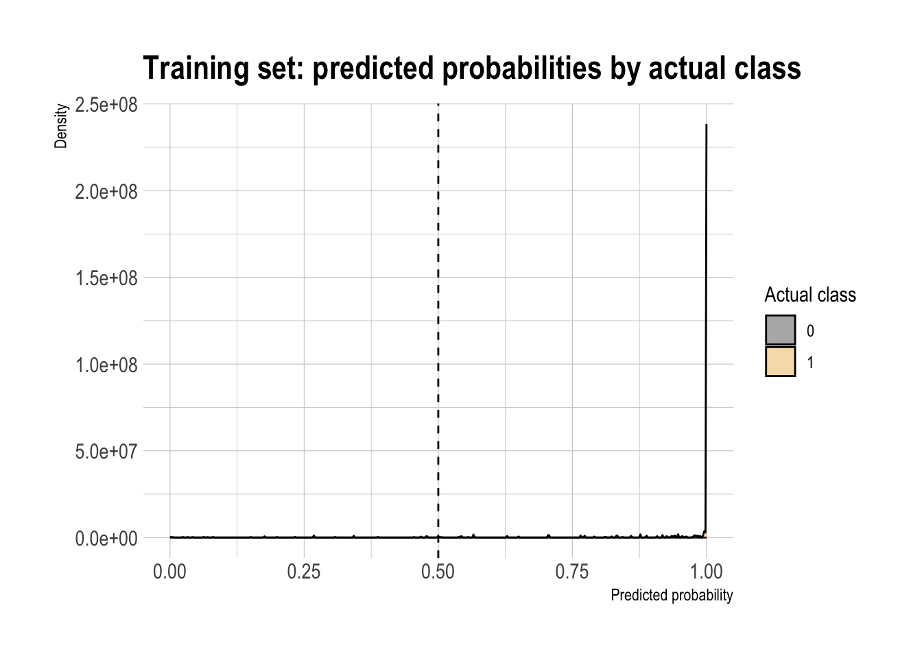
Classification
Double density plot (threshold intuition)
threshold <- 0.5

model |>
  augment(type.predict = "response") |>
  ggplot(aes(x = .fitted,
             fill = factor(fail))) +
  geom_density(alpha = 0.35) +
  geom_vline(xintercept = threshold, linetype = "dashed") +
  labs(
    x = "Predicted probability",
    y = "Density",
    fill = "Actual class",
    title = "Training set: predicted probabilities by actual class"
  )
Confusion Matrix
# threshold <- mean(dtest$fail)
threshold <- 0.5

df_cm <- model |>
  augment(newdata = dtest,
          type.predict = "response") |>
  mutate(
    actual = factor(fail,
                    levels = c(0, 1),
                    labels = c("pass", "fail")),
    pred   = factor(ifelse(.fitted > threshold, 1, 0),
                    levels = c(0, 1),
                    labels = c("pass", "fail"))
  )

conf_mat <- table(truth = df_cm$actual,
                  prediction = df_cm$pred)
conf_mat
prediction
truth pass fail
pass 157 7
fail 17 316# data.frame of confusion matrix
cm_counts <- df_cm |>
group_by(actual, pred) |>
summarize(n = n()) |>
ungroup() |>
pivot_wider(names_from = pred,
values_from = n,
values_fill = 0) |>
rename(`truth / prediction` = actual)
cm_counts# A tibble: 2 × 3
`truth / prediction` pass fail
<fct> <int> <int>
1 pass 157 7
2 fail 17 316Performance Metrics (from conf_mat)
base_rate   <- mean(dtest$fail)

accuracy <- (conf_mat[1,1] + conf_mat[2,2]) / sum(conf_mat)
precision <- conf_mat[2,2] / sum(conf_mat[,2])
recall <- conf_mat[2,2] / sum(conf_mat[2,])
specificity <- conf_mat[1,1] / sum(conf_mat[1,])
enrichment <- precision / base_rate


df_class_metric <-
  data.frame(
    metric = c("Base rate",
               "Accuracy",
               "Precision",
               "Recall",
               "Specificity",
               "Enrichment"),
    value  = c(base_rate,
               accuracy,
               precision,
               recall,
               specificity,
               enrichment)
    )

df_class_metric |>
  mutate(value = round(value, 4)) |>
  rmarkdown::paged_table()
Precision/Recall/Enrichment Curves over Thresholds (using WVPlots package)
plt <- PRTPlot(df_cm,
               ".fitted", "fail", 1,
               plotvars = c("enrichment", "precision", "recall", "specificity", "false_positive_rate"),
               thresholdrange = c(.4,.8),
               title = "With threshold for car safety model")

plt +
  geom_vline(xintercept = threshold,
             color="maroon",
             linetype = 2)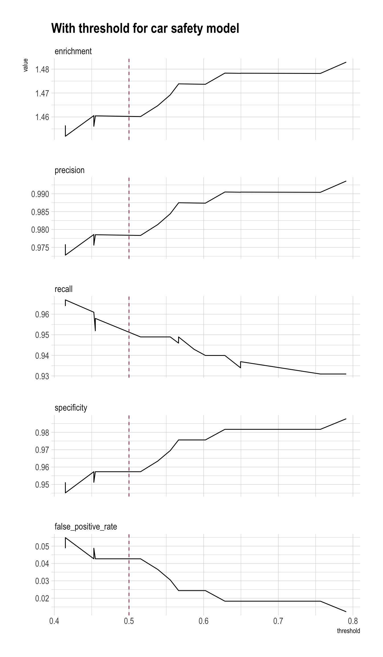
ROC and AUC (using WVPlots and pROC packages)
roc <- ROCPlot(df_cm,
               xvar = '.fitted',
               truthVar = 'fail',
               truthTarget = 1,
               title = 'Classifier performance')

# ROC with vertical line
roc +
  geom_vline(xintercept = 1 - specificity,
             color="maroon", linetype = 2)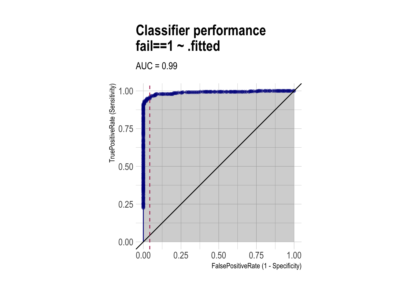
# AUC
# pROC::roc(BINARY_OUTCOME, PREDICTED_PROBABILITY)
roc_obj <- roc(df_cm$fail, df_cm$.fitted)
auc(roc_obj)
Area under the curve: 0.9896Regularized Logistic Regression
Matrices
# fmla <- fail ~ buying + maint + persons + lug_boot + safety

# y must be numeric 0/1 (FALSE->0, TRUE->1)
y_train <- as.integer(dtrain$fail)   # fail is TRUE
y_test  <- as.integer(dtest$fail)

# x must be a numeric matrix
  # [, -1] to remove an intercept variable
X_train <- model.matrix(~ buying + maint + persons + lug_boot + safety, data = dtrain)[, -1]
X_test <- model.matrix(~ buying + maint + persons + lug_boot + safety, data = dtest)[, -1]model.matrix()drops a reference category for each categorical variable in the formula by default.
Fit with cv.glmnet(family = "binomial")
Lasso (alpha = 1)
set.seed(1)
model_lasso <- cv.glmnet(
  X_train, y_train,
  alpha = 1,
  family = "binomial"
)
Ridge (alpha = 0)
set.seed(1)
model_ridge <- cv.glmnet(
  X_train, y_train,
  alpha = 0,
  family = "binomial"
)
Elastic Net (\(0 < \alpha < 1\))
- Loop over alpha values, pick best by min CV deviance:
set.seed(1)

alpha_grid <- seq(0.1, 0.9, by = 0.1)   # 0 < alpha < 1 for elastic net

# for-loop: initial setup
cv_list <- vector("list", length(alpha_grid))
cvm_min <- rep(NA, length(alpha_grid))

for (i in seq_along(alpha_grid)) {
  a <- alpha_grid[i]

  cv_fit <- cv.glmnet(
    X_train, y_train,
    alpha = a,
    family = "binomial"
  )

  cv_list[[i]] <- cv_fit
  cvm_min[i] <- min(cv_fit$cvm)
}

best_i <- which.min(cvm_min)

best_alpha <- alpha_grid[best_i]
model_enet <- cv_list[[best_i]]

best_alpha
[1] 0.3model_enet$lambda.min[1] 5.463574e-05model_enet$lambda.1se[1] 0.001072522\(\lambda\) & CV errors (deviances) with tidy()
CVErrors_lasso <- tidy(model_lasso)
CVErrors_ridge <- tidy(model_ridge)
CVErrors_enet <- tidy(model_enet)
CVErrors_lasso |>
paged_table()CVErrors_ridge |>
paged_table()CVErrors_enet |>
paged_table()lambda: The penalty value \(\,\lambda\,\) used for that row.- Lasso: Larger \(\,\lambda\,\) means stronger shrinkage, so more coefficients become \(0\).
estimate: The mean cross-validated error/loss at that \(\,\lambda\,\) (the average out-of-sample performance across folds).- For
family = "binomial", this is typically mean CV deviance unless you changedtype.measure.
- For
std.error: The standard error of the cross-validated estimate at that \(\,\lambda\,\) across folds.conf.low: The lower bound of the confidence interval for the CV estimate at that \(\,\lambda\,\) (based onconf.level).conf.high: The upper bound of the confidence interval for the CV estimate at that \(\,\lambda\,\) (based onconf.level).nzero: The number of nonzero coefficients at that \(\,\lambda\,\) (how many predictors the lasso keeps; coefficients shrunk to \(0\) are excluded).
\(\lambda_{\text{min}}\) & \(\lambda_{\text{1se}}\) with glance()
lambdas_lasso <- model_lasso |>
  glance()

lambdas_ridge <- model_ridge |>
  glance()

lambdas_enet <- model_enet |>
  glance()
lambdas_lasso |>
paged_table()lambdas_ridge |>
paged_table()lambdas_enet |>
paged_table()Beta Coefficients with coef()
# Logistic
beta <- coef(model)

# Lasso
beta_lasso_1se <- coef(model_lasso,
                       s = "lambda.1se")  # default
beta_lasso_min <- coef(model_lasso,
                       s = "lambda.min")

# Ridge
beta_ridge_1se <- coef(model_ridge)  # default: "lambda.1se"
beta_ridge_min <- coef(model_ridge,
                       s = "lambda.min")

# Elastic net
beta_enet_1se <- coef(model_enet)  # default: "lambda.1se"
beta_enet_min <- coef(model_enet,
                      s = "lambda.min")

betas <- data.frame(
  term = rownames(beta_lasso_1se),
  beta = as.numeric(beta),
  beta_lasso_1se = as.numeric(beta_lasso_1se),
  beta_lasso_min = as.numeric(beta_lasso_min),
  beta_ridge_1se = as.numeric(beta_ridge_1se),
  beta_ridge_min = as.numeric(beta_ridge_min),
  beta_enet_1se = as.numeric(beta_enet_1se),
  beta_enet_min = as.numeric(beta_enet_min)
)

# Show only nonzero in either solution
betas_lasso_nz <- betas |>
  filter(beta_lasso_1se != 0 | beta_lasso_min != 0) |>
  arrange(abs(beta_lasso_1se), abs(beta_lasso_min))
betas |>
paged_table(options =
list(
rows.print = nrow(betas)
)
)Coefficient Plots
One Model
betas |>
  ggplot(aes(x = beta_lasso_1se, y = term)) +
  geom_vline(xintercept = 0,
             color = 'maroon') +
  geom_pointrange(aes(xmin = 0, xmax = beta_lasso_1se)) +
  labs(y = NULL,
       title = "Lasso Logistic Regression (lambda.1se)")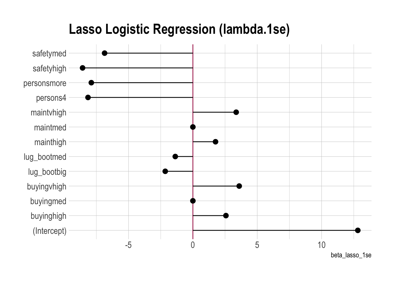
All Models
betas |>
  pivot_longer(cols = beta:beta_enet_min,
               names_to = "model",
               values_to = "value") |>
  ggplot(aes(x = value, y = term, color = model)) +
  geom_vline(xintercept = 0,
             color = 'maroon') +
  geom_pointrange(aes(xmin = 0,
                      xmax = value),
                  position = position_dodge(width = 0.6)) +
  labs(y = NULL) +
  theme(legend.position = "top")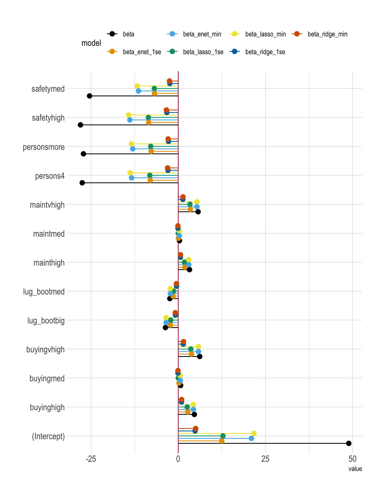
CV curve
# Run all at once

par(mar = c(5.1, 4.1, 6.1, 2.1))  # title margin
plot(model_lasso, main = "Lasso")
abline(v = log(model_lasso$lambda.min), lty = 2)
abline(v = log(model_lasso$lambda.1se), lty = 3)
legend("bottomright",
       legend = c("lambda.min", "lambda.1se"),
       lty = c(2, 3),
       bty = "n")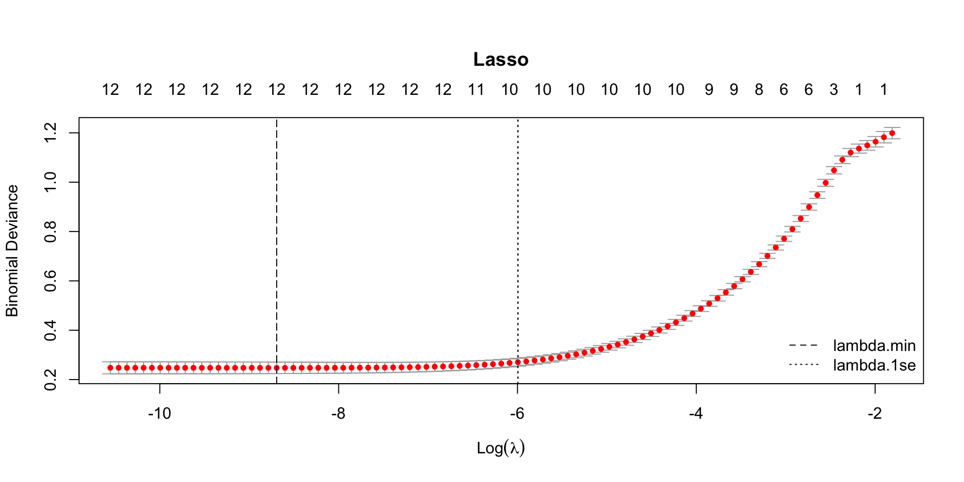
From this plot alone, it’s hard to pinpoint the exact minimum cross-validation (CV) error (binomial deviance) at
lambda.min.
To see the numeric values directly, check the CV results table (e.g.,lasso_CVErrors <- tidy(model_lasso)).We could recreate the CV curve with ggplot2, but the built-in base R
plot()is convenient because it also reports extra diagnostics—especially the number of nonzero coefficients at each value of ().
# Run all at once

par(mar = c(5.1, 4.1, 6.1, 2.1))  # title margin
plot(model_ridge, main = "Ridge")
abline(v = log(model_ridge$lambda.min), lty = 2)
abline(v = log(model_ridge$lambda.1se), lty = 3)
legend("bottomright",
       legend = c("lambda.min", "lambda.1se"),
       lty = c(2, 3),
       bty = "n")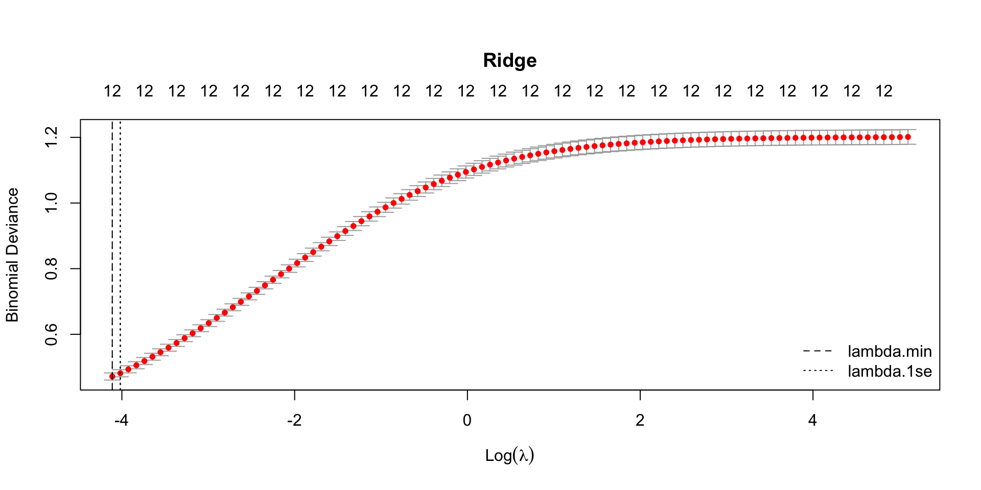
# Run all at once

par(mar = c(5.1, 4.1, 6.1, 2.1))  # title margin
plot(model_enet, main = "Elastic Net")
abline(v = log(model_enet$lambda.min), lty = 2)
abline(v = log(model_enet$lambda.1se), lty = 3)
legend("bottomright",
       legend = c("lambda.min", "lambda.1se"),
       lty = c(2, 3),
       bty = "n")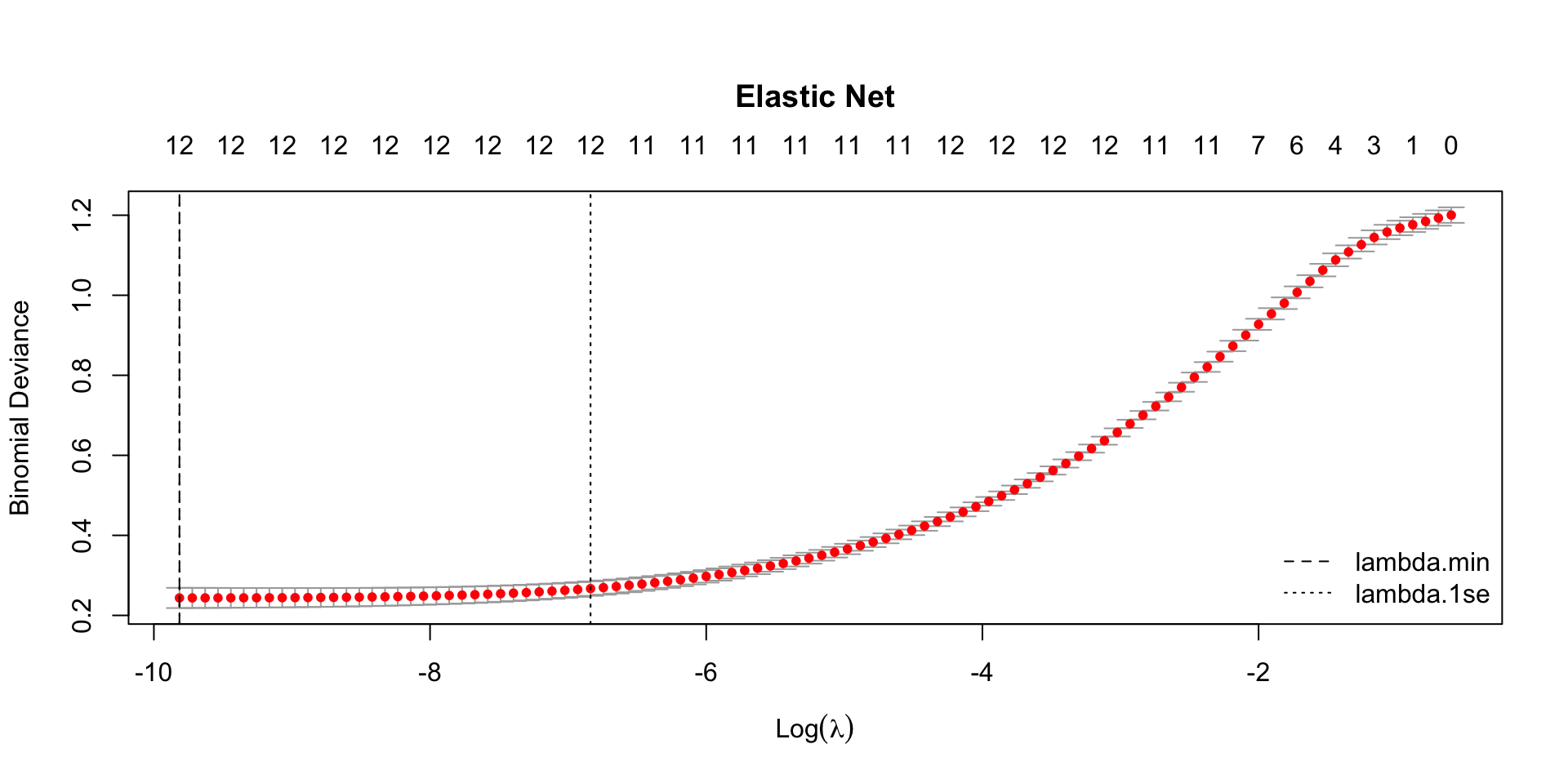
LASSO Coefficient path
# Run all at once

par(mar = c(5.1, 4.1, 6.1, 2.1))  # title margin
plot(model_lasso$glmnet.fit, xvar = "lambda",
     main = "Lasso")
abline(v = log(model_lasso$lambda.min), lty = 2)
abline(v = log(model_lasso$lambda.1se), lty = 3)
legend("topright",
       legend = c("lambda.min", "lambda.1se"),
       lty = c(2, 3),
       bty = "n")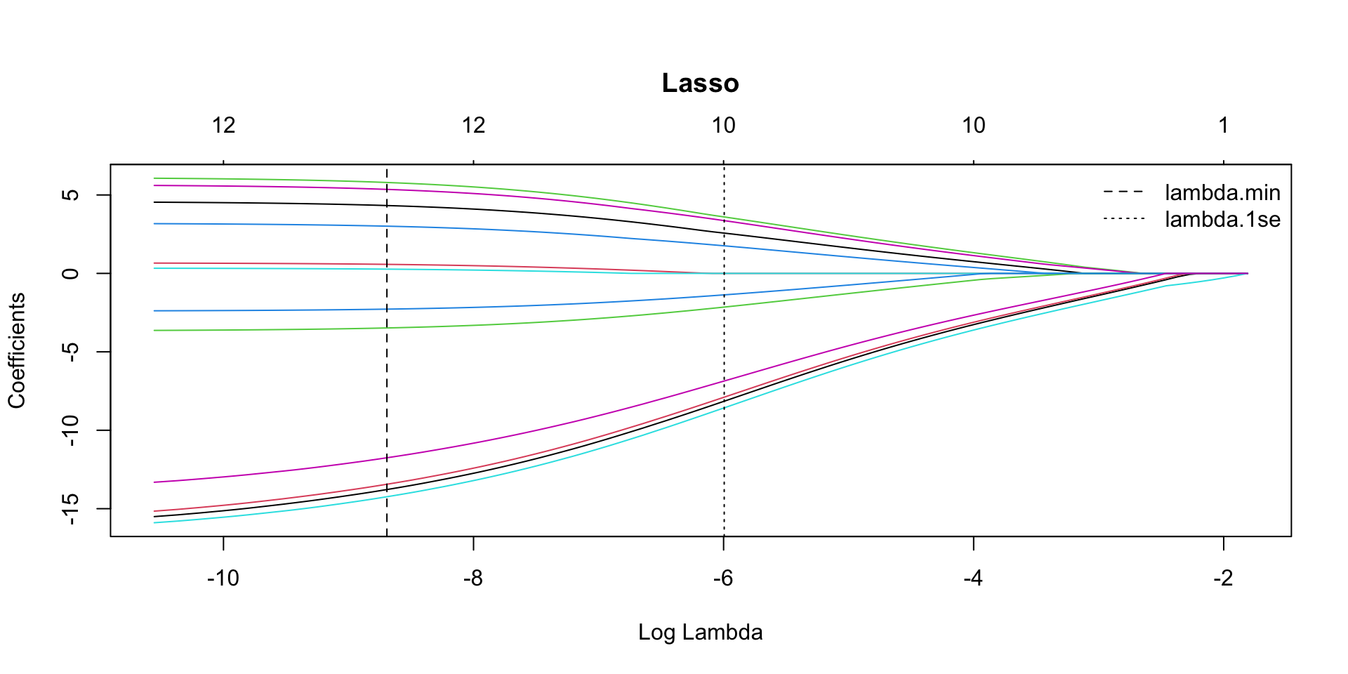
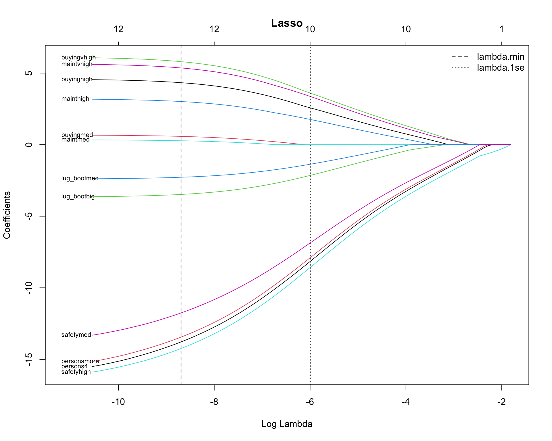
With Predictor Names
# Run all at once

# Coefficient path (keep the default left-to-right order of log(lambda))
fit <- model_lasso$glmnet.fit
B   <- as.matrix(fit$beta)    # p x L (no intercept)
lam <- fit$lambda

x_all <- log(lam)
x_min <- min(x_all)           # smallest log(lambda)
x_max <- max(x_all)

# add extra space to the LEFT (values smaller than the smallest log(lambda))
pad <- 0.6

plot(fit, xvar = "lambda", label = FALSE, main = "Lasso",
     xlim = c(x_min - pad, x_max))
abline(v = log(model_lasso$lambda.min), lty = 2)
abline(v = log(model_lasso$lambda.1se), lty = 3)
legend("topright",
       legend = c("lambda.min", "lambda.1se"),
       lty = c(2, 3),
       bty = "n")

# label at the smallest-lambda end (where curves end)
y_end <- B[, ncol(B)]

# label only a few to avoid clutter
K <- 15  # number of variable names to display
idx <- order(abs(y_end), decreasing = TRUE)[1:min(K, length(y_end))]

# place labels in the extra left margin (x < min log(lambda))
text(
  x      = rep(x_min - 0.75, length(idx)),
  y      = y_end[idx],
  labels = rownames(B)[idx],
  pos    = 4,       # text to the right of the label position
  cex    = 0.7,
  xpd    = NA
)
Classification
Prediction with predict() & Confusion Matrix
# threshold <- mean(dtest$fail)
# threshold <- 0.5

df_cm_all <- dtest |>
  mutate(
    .fitted = predict(model, newdata = dtest,
                      type = "response"),
    .fitted_lasso_1se = predict(model_lasso, newx = X_test,
                                s = "lambda.1se", type = "response"),
    .fitted_lasso_min = predict(model_lasso, newx = X_test,
                                s = "lambda.min", type = "response"),
    .fitted_ridge_1se = predict(model_ridge, newx = X_test,
                                s = "lambda.1se", type = "response"),
    .fitted_ridge_min = predict(model_ridge, newx = X_test,
                                s = "lambda.min", type = "response"),
    .fitted_enet_1se = predict(model_enet, newx = X_test,
                               s = "lambda.1se", type = "response"),
    .fitted_enet_min = predict(model_enet, newx = X_test,
                               s = "lambda.min", type = "response")
  ) |>
  mutate(
    actual = factor(fail,
                    levels = c(0, 1),
                    labels = c("pass", "fail")),
    pred   = factor(ifelse(.fitted > threshold, 1, 0),
                    levels = c(0, 1),
                    labels = c("pass", "fail")),
    pred_lasso   = factor(ifelse(.fitted_lasso_1se > threshold, 1, 0),
                          levels = c(0, 1),
                          labels = c("pass", "fail")),
    pred_ridge   = factor(ifelse(.fitted_ridge_1se > threshold, 1, 0),
                          levels = c(0, 1),
                          labels = c("pass", "fail")),
    pred_enet   = factor(ifelse(.fitted_enet_1se > threshold, 1, 0),
                         levels = c(0, 1),
                         labels = c("pass", "fail"))
  )
# Logistic
conf_mat <- table(truth = df_cm_all$actual,
prediction_logitstic = df_cm_all$pred)
conf_mat prediction_logitstic
truth pass fail
pass 157 7
fail 17 316# Lasso Logistic
conf_mat_lasso <- table(truth = df_cm_all$actual,
prediction_lasso = df_cm_all$pred_lasso)
conf_mat_lasso prediction_lasso
truth pass fail
pass 156 8
fail 15 318# Ridge Logistic
conf_mat_ridge <- table(truth = df_cm_all$actual,
prediction_ridge = df_cm_all$pred_ridge)
conf_mat_ridge prediction_ridge
truth pass fail
pass 144 20
fail 10 323# Elastic Net Logistic
conf_mat_enet <- table(truth = df_cm_all$actual,
prediction_enet = df_cm_all$pred_enet)
conf_mat_enet prediction_enet
truth pass fail
pass 157 7
fail 17 316Performance Metrics (from conf_mat)
base_rate   <- mean(dtest$fail)

# Logistic
accuracy <- (conf_mat[1,1] + conf_mat[2,2]) / sum(conf_mat)
precision <- conf_mat[2,2] / sum(conf_mat[,2])
recall <- conf_mat[2,2] / sum(conf_mat[2,])
specificity <- conf_mat[1,1] / sum(conf_mat[1,])
enrichment <- precision / base_rate

# Lasso Logistic
accuracy_lasso <- (conf_mat_lasso[1,1] + conf_mat_lasso[2,2]) / sum(conf_mat_lasso)
precision_lasso <- conf_mat_lasso[2,2] / sum(conf_mat_lasso[,2])
recall_lasso <- conf_mat_lasso[2,2] / sum(conf_mat_lasso[2,])
specificity_lasso <- conf_mat_lasso[1,1] / sum(conf_mat_lasso[1,])
enrichment_lasso <- precision_lasso / base_rate

# Ridge Logistic
accuracy_ridge <- (conf_mat_ridge[1,1] + conf_mat_ridge[2,2]) / sum(conf_mat_ridge)
precision_ridge <- conf_mat_ridge[2,2] / sum(conf_mat_ridge[,2])
recall_ridge <- conf_mat_ridge[2,2] / sum(conf_mat_ridge[2,])
specificity_ridge <- conf_mat_ridge[1,1] / sum(conf_mat_ridge[1,])
enrichment_ridge <- precision_ridge / base_rate

# Elastic Net Logistic
accuracy_enet <- (conf_mat_enet[1,1] + conf_mat_enet[2,2]) / sum(conf_mat_enet)
precision_enet <- conf_mat_enet[2,2] / sum(conf_mat_enet[,2])
recall_enet <- conf_mat_enet[2,2] / sum(conf_mat_enet[2,])
specificity_enet <- conf_mat_enet[1,1] / sum(conf_mat_enet[1,])
enrichment_enet <- precision_enet / base_rate


df_class_metric <-
  data.frame(
    metric = c("Base rate",
               "Accuracy",
               "Precision",
               "Recall",
               "Specificity",
               "Enrichment"),
    value_logistic  = c(base_rate,
                        accuracy,
                        precision,
                        recall,
                        specificity,
                        enrichment),
    value_lasso  = c(base_rate,
                     accuracy_lasso,
                     precision_lasso,
                     recall_lasso,
                     specificity_lasso,
                     enrichment_lasso),
    value_ridge  = c(base_rate,
                     accuracy_ridge,
                     precision_ridge,
                     recall_ridge,
                     specificity_ridge,
                     enrichment_ridge),
    value_enet  = c(base_rate,
                    accuracy_enet,
                    precision_enet,
                    recall_enet,
                    specificity_enet,
                    enrichment_enet)
    )

df_class_metric |>
  mutate(value_logistic = round(value_logistic, 4),
         value_lasso = round(value_lasso, 4),
         value_ridge = round(value_ridge, 4),
         value_enet = round(value_enet, 4)
         ) |>
  rmarkdown::paged_table()
Precision/Recall/Enrichment Curves over Thresholds (using WVPlots package)
plt <- PRTPlot(df_cm_all,
               ".fitted", "fail", 1,
               plotvars = c("enrichment", "precision", "recall", "specificity", "false_positive_rate"),
               thresholdrange = c(.4,.8),
               title = "With threshold for Logistic Regression Model")

plt +
  geom_vline(xintercept = threshold,
             color="maroon",
             linetype = 2)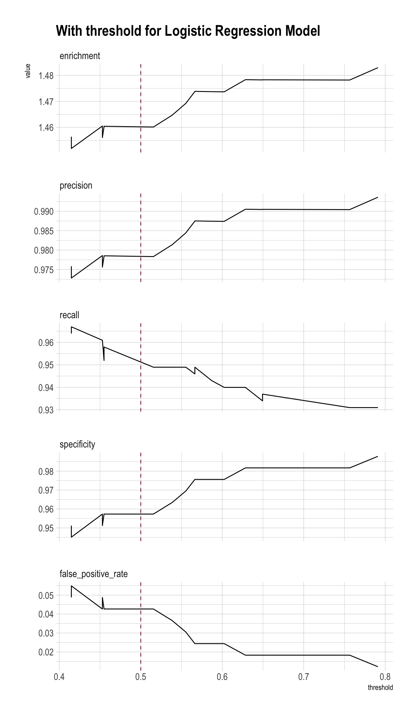
plt_lasso <- PRTPlot(df_cm_all,
               ".fitted_lasso_1se", "fail", 1,
               plotvars = c("enrichment", "precision", "recall", "specificity", "false_positive_rate"),
               thresholdrange = c(.4,.8),
               title = "With threshold for Lasso Logistic Regression Model")

plt_lasso +
  geom_vline(xintercept = threshold,
             color="maroon",
             linetype = 2)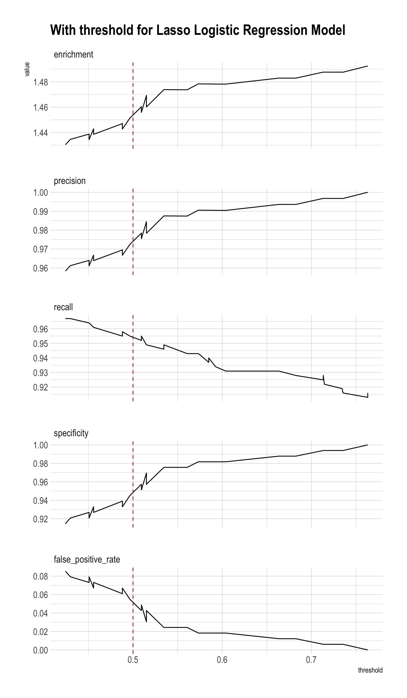
plt_ridge <- PRTPlot(df_cm_all,
               ".fitted_ridge_1se", "fail", 1,
               plotvars = c("enrichment", "precision", "recall", "specificity", "false_positive_rate"),
               thresholdrange = c(.4,.8),
               title = "With threshold for Ridge Logistic Regression Model")

plt_ridge +
  geom_vline(xintercept = threshold,
             color="maroon",
             linetype = 2)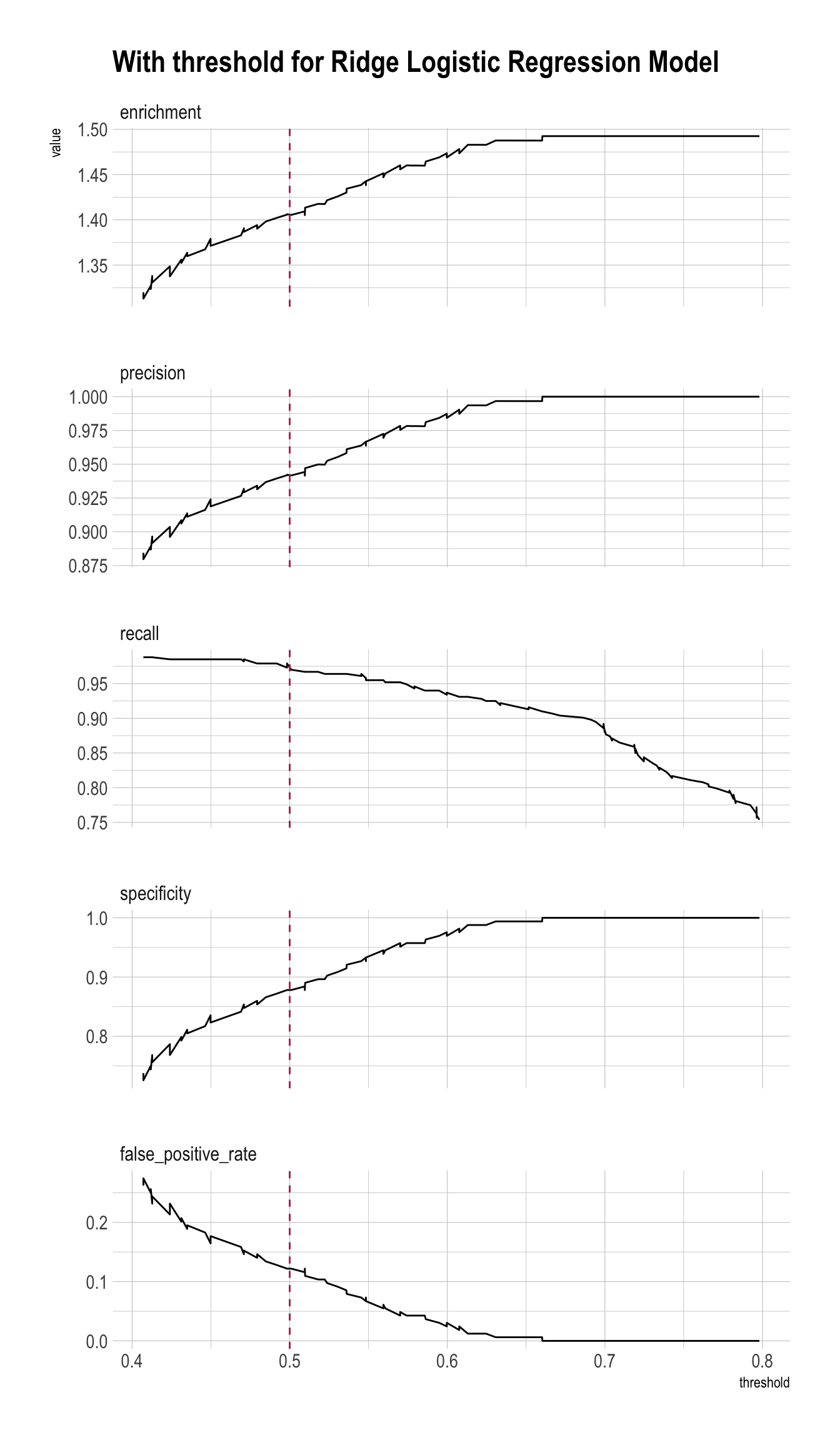
plt_enet <- PRTPlot(df_cm_all,
               ".fitted_enet_1se", "fail", 1,
               plotvars = c("enrichment", "precision", "recall", "specificity", "false_positive_rate"),
               thresholdrange = c(.4,.8),
               title = "With threshold for Elastic Net Logistic Regression Model")

plt_enet +
  geom_vline(xintercept = threshold,
             color="maroon",
             linetype = 2)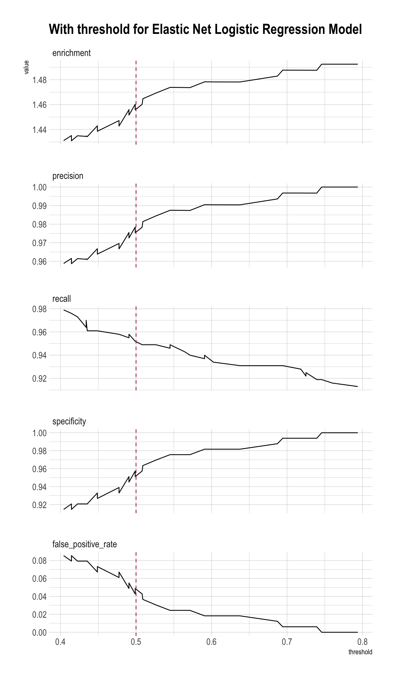
ROC (using WVPlots package)
roc <- ROCPlot(df_cm_all,
               xvar = '.fitted',
               truthVar = 'fail',
               truthTarget = 1,
               title = 'Logistic Regression Model')

# ROC with vertical line
roc +
  geom_vline(xintercept = 1 - specificity,
             color="maroon", linetype = 2)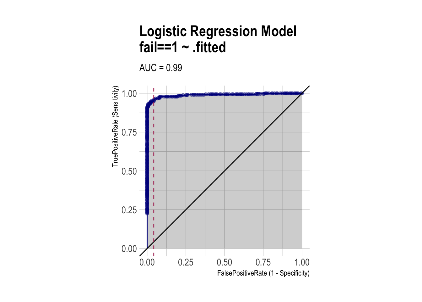
roc_lasso <- ROCPlot(df_cm_all,
                     xvar = '.fitted_lasso_1se',
                     truthVar = 'fail',
                     truthTarget = 1,
                     title = 'Lasso Logistic Regression Model')

# ROC with vertical line
roc_lasso +
  geom_vline(xintercept = 1 - specificity_lasso,
             color="maroon", linetype = 2)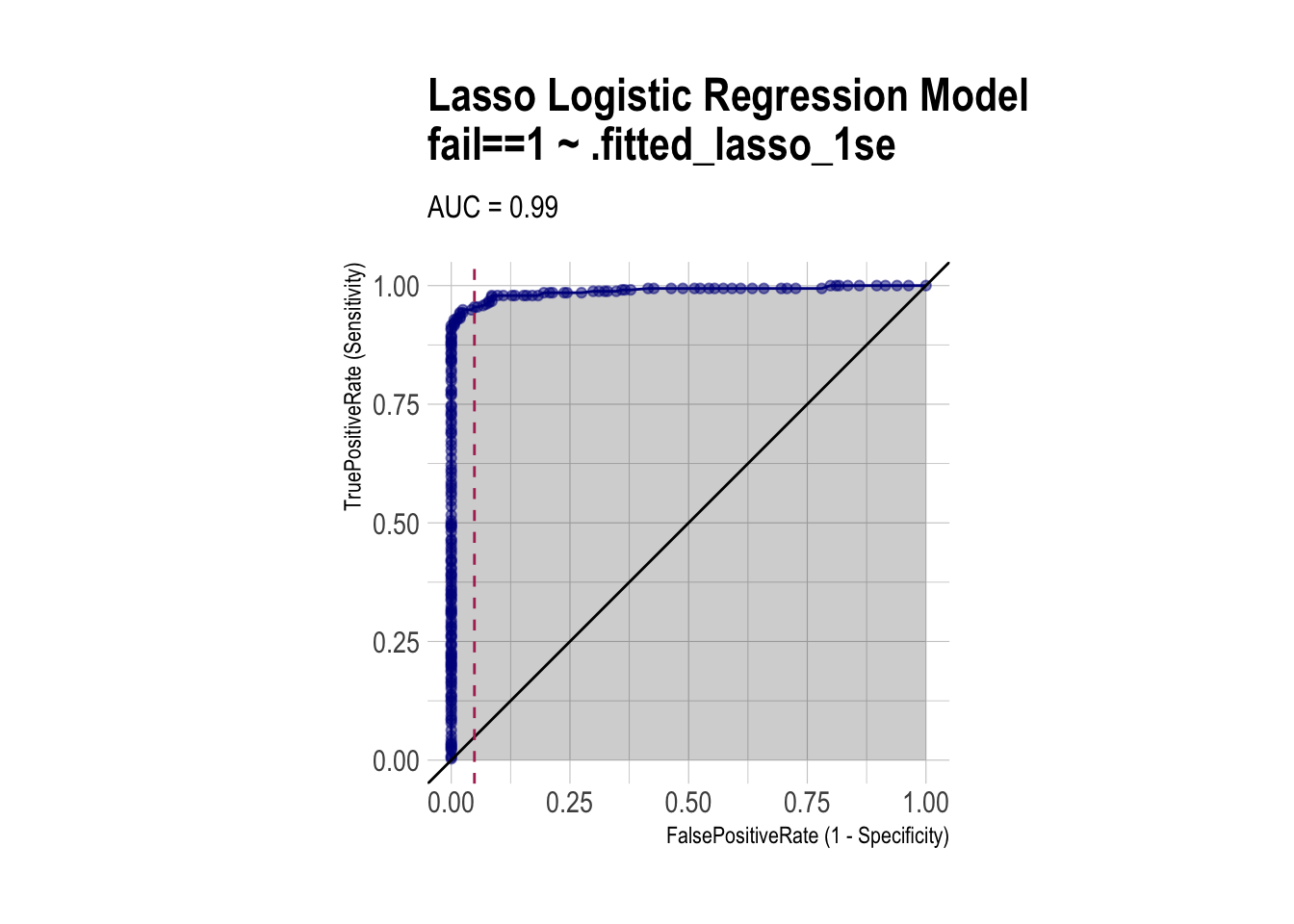
roc_ridge <- ROCPlot(df_cm_all,
                     xvar = '.fitted_ridge_1se',
                     truthVar = 'fail',
                     truthTarget = 1,
                     title = 'Ridge Logistic Regression Model')

# ROC with vertical line
roc_ridge +
  geom_vline(xintercept = 1 - specificity_ridge,
             color="maroon", linetype = 2)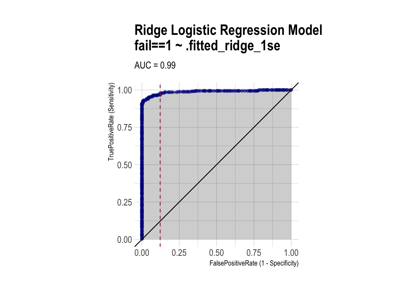
roc_enet <- ROCPlot(df_cm_all,
                     xvar = '.fitted_enet_1se',
                     truthVar = 'fail',
                     truthTarget = 1,
                     title = 'Elastic Net Logistic Regression Model')

# ROC with vertical line
roc_enet +
  geom_vline(xintercept = 1 - specificity_enet,
             color="maroon", linetype = 2)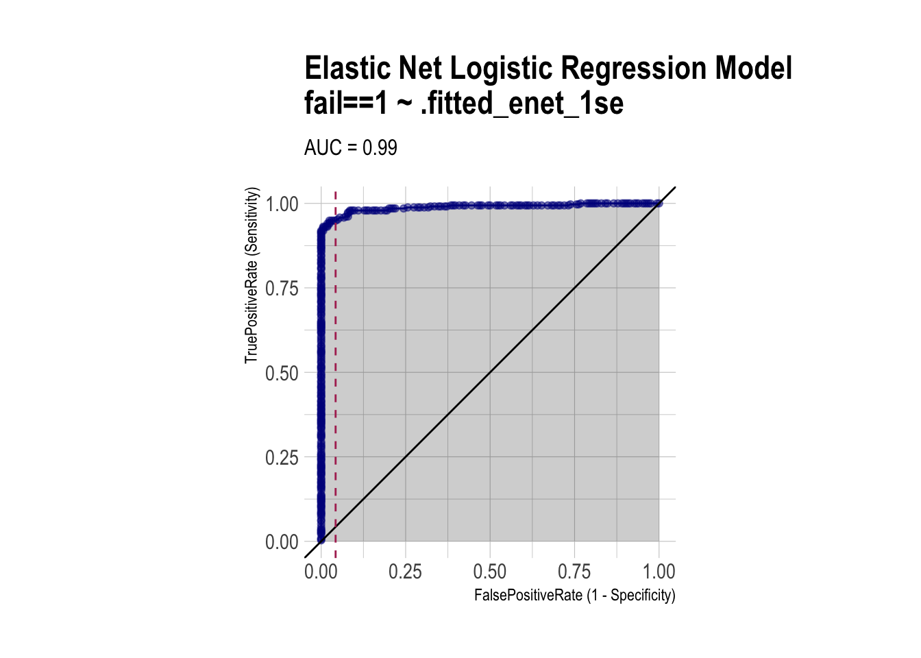
AUC (using pROC package)
# ROC objects
roc_logit <- roc(df_cm_all$fail, df_cm_all$.fitted)
roc_lasso <- roc(df_cm_all$fail, df_cm_all$.fitted_lasso_1se)
roc_ridge <- roc(df_cm_all$fail, df_cm_all$.fitted_ridge_1se)
roc_enet  <- roc(df_cm_all$fail, df_cm_all$.fitted_enet_1se)


auc_df <- data.frame(
  model = c("Logistic", "Lasso (lambda.1se)", "Ridge (lambda.1se)", "Elastic Net (lambda.1se)"),
  auc   = c(
    as.numeric(auc(roc_logit)),
    as.numeric(auc(roc_lasso)),
    as.numeric(auc(roc_ridge)),
    as.numeric(auc(roc_enet))
  )
)

auc_df |>
  arrange(-auc) |>
  paged_table()