boston <- read_csv("https://bcdanl.github.io/data/boston.csv") |>
  janitor::clean_names()

paged_table(boston)Pruning Trees
Boston Housing Data
Pruning with Boston Housing Data
Boston Housing Data
- Boston housing is a classic regression example with multiple socioeconomic and neighborhood predictors
| Variable | Description |
|---|---|
crim |
Per capita crime rate by town |
zn |
Proportion of residential land zoned for lots over 25,000 sq.ft. |
indus |
Proportion of non-retail business acres per town |
chas |
Charles River dummy variable (= 1 if tract bounds river; 0 otherwise) |
nox |
Nitrogen oxides concentration (parts per 10 million) |
rm |
Average number of rooms per dwelling |
age |
Proportion of owner-occupied units built prior to 1940 |
dis |
Weighted mean of distances to five Boston employment centres |
rad |
Index of accessibility to radial highways |
tax |
Full-value property-tax rate per $10,000 |
ptratio |
Pupil-teacher ratio by town |
black |
Proportion of Black residents by town |
lstat |
Lower socioeconomic status of the population (percent) |
medv |
Median value of owner-occupied homes in $1000s |
Modeling goal
- Predict
medv, median housing value in thousands of dollars - We will use it to study pruning
Create training and test data
set.seed(42120532)
boston <- boston |>
  mutate(rnd = runif(n()))

dtrain <- boston |>
  filter(rnd > .2) |>
  select(-rnd)

dtest <- boston |>
  filter(rnd <= .2) |>
  select(-rnd)

x_train <- dtrain |> select(-medv)
y_train <- dtrain$medv
x_test  <- dtest |> select(-medv)
y_test  <- dtest$medv
Fit an initial Boston regression tree
boston_tree <- rpart(
  medv ~ .,
  data = dtrain,
  method = "anova",
  control = rpart.control(cp = 0, xval = 10, minsplit = 10)
)

boston_tree
n= 392
node), split, n, deviance, yval
* denotes terminal node
1) root 392 3.264805e+04 22.422960
2) lstat>=9.725 230 5.391070e+03 17.260430
4) lstat>=14.915 133 2.457224e+03 14.783460
8) nox>=0.603 83 1.006908e+03 12.912050
16) lstat>=19.645 43 3.891963e+02 10.690700
32) tax>=551.5 36 2.398156e+02 9.911111
64) dis>=1.40575 30 1.542667e+02 9.233333
128) dis< 1.85045 23 8.361478e+01 8.439130
256) nox< 0.6965 13 2.816769e+01 7.569231
512) lstat>=22.03 8 9.738750e+00 6.837500 *
513) lstat< 22.03 5 7.292000e+00 8.740000 *
257) nox>=0.6965 10 3.282100e+01 9.570000
514) crim>=11.6951 7 9.620000e+00 8.700000 *
515) crim< 11.6951 3 5.540000e+00 11.600000 *
129) dis>=1.85045 7 8.477143e+00 11.842860 *
65) dis< 1.40575 6 2.860000e+00 13.300000 *
33) tax< 551.5 7 1.498000e+01 14.700000 *
17) lstat< 19.645 40 1.774400e+02 15.300000
34) crim>=12.2236 3 2.660000e+00 11.600000 *
35) crim< 12.2236 37 1.303800e+02 15.600000
70) lstat>=17.665 14 3.010929e+01 14.607140
140) black< 329.75 4 3.087500e+00 13.675000 *
141) black>=329.75 10 2.215600e+01 14.980000
282) age< 96.95 4 4.050000e+00 14.150000 *
283) age>=96.95 6 1.351333e+01 15.533330 *
71) lstat< 17.665 23 7.806957e+01 16.204350
142) crim>=6.192045 9 2.648000e+01 15.200000 *
143) crim< 6.192045 14 3.667500e+01 16.850000
286) rm< 5.701 3 5.406667e+00 14.966670 *
287) rm>=5.701 11 1.772545e+01 17.363640
574) age< 98.45 8 1.038000e+01 16.900000 *
575) age>=98.45 3 1.040000e+00 18.600000 *
9) nox< 0.603 50 6.771050e+02 17.890000
18) crim>=0.592985 20 2.698300e+02 15.450000
36) dis>=1.57165 16 9.225000e+01 14.325000
72) age< 83 3 4.500000e+00 11.700000 *
73) age>=83 13 6.230769e+01 14.930770
146) black< 385.45 10 3.360400e+01 14.340000
292) dis>=3.15005 5 8.720000e-01 13.360000 *
293) dis< 3.15005 5 2.312800e+01 15.320000 *
147) black>=385.45 3 1.358000e+01 16.900000 *
37) dis< 1.57165 4 7.633000e+01 19.950000 *
19) crim< 0.592985 30 2.088217e+02 19.516670
38) age>=55.9 27 1.659667e+02 19.122220
76) lstat>=24.25 4 4.587500e+00 15.975000 *
77) lstat< 24.25 23 1.148687e+02 19.669570
154) age< 95.95 20 5.663800e+01 19.290000
308) indus< 10.3 14 2.638929e+01 18.607140
616) lstat>=18.73 3 1.142000e+01 17.100000 *
617) lstat< 18.73 11 6.296364e+00 19.018180
1234) age>=73.3 7 2.774286e+00 18.728570 *
1235) age< 73.3 4 1.907500e+00 19.525000 *
309) indus>=10.3 6 8.488333e+00 20.883330 *
155) age>=95.95 3 3.614000e+01 22.200000 *
39) age< 55.9 3 8.466667e-01 23.066670 *
5) lstat< 14.915 97 9.989781e+02 20.656700
10) indus>=3.985 91 6.639246e+02 20.292310
20) crim>=16.9714 3 1.120667e+01 13.633330 *
21) crim< 16.9714 88 5.151572e+02 20.519320
42) rm< 6.0565 50 2.943218e+02 19.858000
84) black>=336.845 44 1.868600e+02 19.500000
168) black< 376.91 6 1.469500e+01 17.250000 *
169) black>=376.91 38 1.369939e+02 19.855260
338) indus< 10.3 27 9.631185e+01 19.274070
676) ptratio>=16.75 24 6.629958e+01 18.979170
1352) rm< 5.729 6 6.108333e+00 17.783330 *
1353) rm>=5.729 18 4.875111e+01 19.377780
2706) age>=45.85 15 1.661733e+01 18.946670
5412) lstat>=13.965 4 2.527500e+00 17.875000 *
5413) lstat< 13.965 11 7.825455e+00 19.336360
10826) dis>=5.42305 3 8.266667e-01 18.233330 *
10827) dis< 5.42305 8 1.980000e+00 19.750000 *
2707) age< 45.85 3 1.540667e+01 21.533330 *
677) ptratio< 16.75 3 1.122667e+01 21.633330 *
339) indus>=10.3 11 9.176364e+00 21.281820
678) tax>=534.5 5 1.948000e+00 20.680000 *
679) tax< 534.5 6 3.908333e+00 21.783330 *
85) black< 336.845 6 6.046833e+01 22.483330 *
43) rm>=6.0565 38 1.701958e+02 21.389470
86) ptratio>=17.6 30 9.375367e+01 20.856670
172) black< 363.395 3 7.460000e+00 18.200000 *
173) black>=363.395 27 6.276741e+01 21.151850
346) age>=83.8 10 1.681600e+01 20.020000
692) black>=387.815 7 2.677143e+00 19.342860 *
693) black< 387.815 3 3.440000e+00 21.600000 *
347) age< 83.8 17 2.560471e+01 21.817650
694) rm< 6.3215 13 1.143077e+01 21.338460
1388) rm>=6.2455 3 1.486667e+00 20.433330 *
1389) rm< 6.2455 10 6.749000e+00 21.610000
2778) ptratio< 19.65 5 3.520000e-01 20.940000 *
2779) ptratio>=19.65 5 1.908000e+00 22.280000 *
695) rm>=6.3215 4 1.487500e+00 23.375000 *
87) ptratio< 17.6 8 3.598875e+01 23.387500 *
11) indus< 3.985 6 1.397083e+02 26.183330 *
3) lstat< 9.725 162 1.242418e+04 29.752470
6) rm< 6.978 113 4.092169e+03 25.871680
12) dis>=1.557 109 1.678009e+03 24.986240
24) rm< 6.543 65 3.401514e+02 22.816920
48) rm< 6.1245 24 5.938958e+01 21.070830
96) rm< 6.062 15 2.493733e+01 20.386670
192) crim< 0.072155 6 6.468333e+00 19.483330 *
193) crim>=0.072155 9 1.030889e+01 20.988890 *
97) rm>=6.062 9 1.572889e+01 22.211110 *
49) rm>=6.1245 41 1.647576e+02 23.839020
98) rad< 1.5 3 2.400667e+01 20.466670 *
99) rad>=1.5 38 1.039389e+02 24.105260
198) ptratio>=19.65 5 1.014800e+01 22.680000 *
199) ptratio< 19.65 33 8.209515e+01 24.321210
398) tax>=245 28 5.868679e+01 24.060710
796) lstat< 9.21 24 4.011833e+01 23.841670
1592) rad< 6.5 21 3.155238e+01 23.647620
3184) lstat>=7.72 6 5.573333e+00 22.566670 *
3185) lstat< 7.72 15 1.616400e+01 24.080000
6370) age< 31.75 8 1.840000e+00 23.400000 *
6371) age>=31.75 7 6.397143e+00 24.857140 *
1593) rad>=6.5 3 2.240000e+00 25.200000 *
797) lstat>=9.21 4 1.050750e+01 25.375000 *
399) tax< 245 5 1.086800e+01 25.780000 *
25) rm>=6.543 44 5.800964e+02 28.190910
50) lstat>=5.195 29 2.051331e+02 26.775860
100) indus>=4.455 17 7.560118e+01 25.741180
200) ptratio>=16.5 14 5.314857e+01 25.228570
400) indus>=9.23 4 2.450000e+00 23.350000 *
401) indus< 9.23 10 3.093600e+01 25.980000
802) rm< 6.6785 4 2.047500e+00 24.275000 *
803) rm>=6.6785 6 9.508333e+00 27.116670 *
201) ptratio< 16.5 3 1.606667e+00 28.133330 *
101) indus< 4.455 12 8.554917e+01 28.241670
202) nox< 0.436 4 3.660000e+00 25.000000 *
203) nox>=0.436 8 1.883875e+01 29.862500 *
51) lstat< 5.195 15 2.046293e+02 30.926670
102) zn< 19 3 4.446000e+01 26.100000 *
103) zn>=19 12 7.280667e+01 32.133330
206) nox< 0.434 5 6.028000e+00 30.180000 *
207) nox>=0.434 7 3.407429e+01 33.528570 *
13) dis< 1.557 4 0.000000e+00 50.000000 *
7) rm>=6.978 49 2.705530e+03 38.702040
14) rm< 7.445 28 4.584171e+02 34.071430
28) age< 86.7 25 1.786200e+02 33.260000
56) nox>=0.4885 5 4.586800e+01 30.120000 *
57) nox< 0.4885 20 7.112950e+01 34.045000
114) black< 390.46 4 1.245000e+01 32.050000 *
115) black>=390.46 16 3.877937e+01 34.543750
230) rad< 2.5 6 5.095000e+00 33.450000 *
231) rad>=2.5 10 2.220000e+01 35.200000
462) indus< 2.32 5 7.752000e+00 34.260000 *
463) indus>=2.32 5 5.612000e+00 36.140000 *
29) age>=86.7 3 1.261667e+02 40.833330 *
15) rm>=7.445 21 8.461981e+02 44.876190
30) ptratio>=17.6 3 2.554067e+02 34.833330 *
31) ptratio< 17.6 18 2.377850e+02 46.550000
62) crim< 1.019325 15 1.949360e+02 45.860000
124) crim>=0.02093 12 1.306625e+02 44.825000
248) lstat< 3.46 5 3.754800e+01 42.220000 *
249) lstat>=3.46 7 3.494857e+01 46.685710 *
125) crim< 0.02093 3 0.000000e+00 50.000000 *
63) crim>=1.019325 3 0.000000e+00 50.000000 *rpart.plot(boston_tree, tweak = 0.8)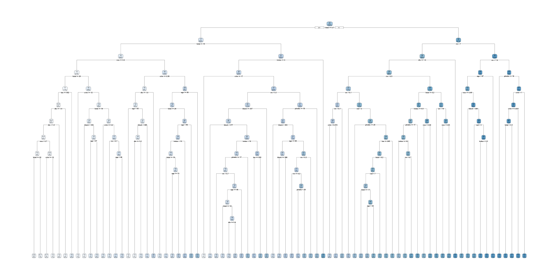
plotcp(boston_tree)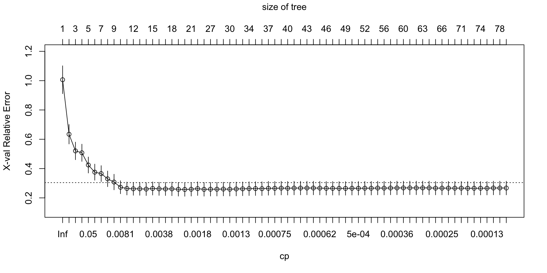
Interpreting the Boston tree
- The tree is segmenting neighborhoods into groups with similar median housing values.
- Splits near the top often involve predictors with strong explanatory value for house prices.
- Each leaf gives a mean
medvfor the neighborhoods in that terminal region. - A large tree may capture complex heterogeneity, but it can also overfit the training sample.
Cost-complexity pruning path
cp_table_boston <- boston_tree$cptable |>
  as_tibble()

cp_table_boston |>
  paged_table()
Select the pruning parameter (with or without the 1-SE rule)
min_xerror_boston <- min(cp_table_boston$xerror)
min_row_boston <- cp_table_boston |>
  filter(xerror == min_xerror_boston) |>
  slice(1)

# 1-SE rule
# xerror_threshold_boston <- min_row_boston$xerror + min_row_boston$xstd

xerror_threshold_boston <- min_row_boston$xerror

cp_1se_boston <- cp_table_boston |>
  filter(CP > 0, xerror <= xerror_threshold_boston) |>
  arrange(nsplit) |>
  slice(1) |>
  pull(CP)

pruned_boston_tree <- prune(boston_tree, cp = cp_1se_boston)

cp_1se_boston
[1] 0.001904394pruned_boston_treen= 392
node), split, n, deviance, yval
* denotes terminal node
1) root 392 32648.05000 22.422960
2) lstat>=9.725 230 5391.07000 17.260430
4) lstat>=14.915 133 2457.22400 14.783460
8) nox>=0.603 83 1006.90800 12.912050
16) lstat>=19.645 43 389.19630 10.690700
32) tax>=551.5 36 239.81560 9.911111
64) dis>=1.40575 30 154.26670 9.233333 *
65) dis< 1.40575 6 2.86000 13.300000 *
33) tax< 551.5 7 14.98000 14.700000 *
17) lstat< 19.645 40 177.44000 15.300000 *
9) nox< 0.603 50 677.10500 17.890000
18) crim>=0.592985 20 269.83000 15.450000
36) dis>=1.57165 16 92.25000 14.325000 *
37) dis< 1.57165 4 76.33000 19.950000 *
19) crim< 0.592985 30 208.82170 19.516670 *
5) lstat< 14.915 97 998.97810 20.656700
10) indus>=3.985 91 663.92460 20.292310
20) crim>=16.9714 3 11.20667 13.633330 *
21) crim< 16.9714 88 515.15720 20.519320 *
11) indus< 3.985 6 139.70830 26.183330 *
3) lstat< 9.725 162 12424.18000 29.752470
6) rm< 6.978 113 4092.16900 25.871680
12) dis>=1.557 109 1678.00900 24.986240
24) rm< 6.543 65 340.15140 22.816920
48) rm< 6.1245 24 59.38958 21.070830 *
49) rm>=6.1245 41 164.75760 23.839020 *
25) rm>=6.543 44 580.09640 28.190910
50) lstat>=5.195 29 205.13310 26.775860 *
51) lstat< 5.195 15 204.62930 30.926670
102) zn< 19 3 44.46000 26.100000 *
103) zn>=19 12 72.80667 32.133330 *
13) dis< 1.557 4 0.00000 50.000000 *
7) rm>=6.978 49 2705.53000 38.702040
14) rm< 7.445 28 458.41710 34.071430
28) age< 86.7 25 178.62000 33.260000 *
29) age>=86.7 3 126.16670 40.833330 *
15) rm>=7.445 21 846.19810 44.876190
30) ptratio>=17.6 3 255.40670 34.833330 *
31) ptratio< 17.6 18 237.78500 46.550000 *rpart.plot(pruned_boston_tree, tweak = 0.9)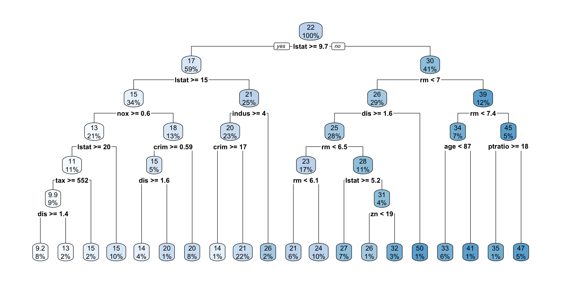
Cross-validation and pruning
- Cross-validation compares candidate subtrees using out-of-sample performance.
- In
rpart, the CP table summarizes this comparison. - The key quantities are:
nsplit: the number of splitsrel error: relative training errorxerror: cross-validated errorxstd: standard error of the cross-validated error
- The tree with the smallest
xerroris the one with the best estimated cross-validated performance.
Why & How to use the 1-SE rule?
- Look for the tree size with the smallest cross-validated error.
- A common rule is the 1-SE rule:
- find the minimum
xerror - then choose the simplest tree whose
xerroris within one standard error of that minimum
- find the minimum
- This favors a smaller, more interpretable tree when its performance is close to the best-performing tree.
- The minimum
xerrorrule can still choose a fairly complex tree. - The 1-SE rule chooses the simplest tree whose cross-validated error is still close to the minimum.
- This is often a better teaching example because it highlights the trade-off between fit and interpretability.
- It also makes it easier to see that pruning can materially simplify the tree.
Compare full and pruned Boston trees
train_pred_tree_full <- predict(boston_tree, newdata = dtrain)
test_pred_tree_full  <- predict(boston_tree, newdata = dtest)

train_pred_tree_pruned <- predict(pruned_boston_tree, newdata = dtrain)
test_pred_tree_pruned  <- predict(pruned_boston_tree, newdata = dtest)

df_rmse <- tibble(
  model = c("Full regression tree", "Pruned regression tree"),
  train_rmse = c(
    sqrt(mean((y_train - train_pred_tree_full)^2)),
    sqrt(mean((y_train - train_pred_tree_pruned)^2))
  ),
  test_rmse = c(
    sqrt(mean((y_test - test_pred_tree_full)^2)),
    sqrt(mean((y_test - test_pred_tree_pruned)^2))
  )
)

df_rmse |>
  paged_table()
Why compare training and test error?
- Training error usually decreases as the tree becomes more complex and adds more splits.
- Test error tells us how well the model predicts outcomes for new, unseen data.
- If training error keeps falling but test error stops improving or starts increasing, the tree may be overfitting the training data.
- Pruning helps control model complexity so the tree can generalize better rather than just fit noise in the training sample.