library(tidyverse)
library(broom)
library(stargazer)
library(margins)
library(yardstick)
library(WVPlots)
library(pROC)
library(DT)
library(rmarkdown)
library(hrbrthemes)
library(ggthemes)

theme_set(
  theme_ipsum()
)

scale_colour_discrete <- function(...) scale_color_colorblind(...)
scale_fill_discrete <- function(...) scale_fill_colorblind(...)Logistic Regression
Newborn Babies
R Packages and Settings
Data: NatalRiskData
df <- read_csv("https://bcdanl.github.io/data/NatalRiskData.csv")
paged_table(df)| Variable | Type | Description |
|---|---|---|
atRisk |
Bool | 1 if Apgar < 7, 0 otherwise |
PWGT |
Num | Prepregnancy weight |
UPREVIS |
Int | Prenatal visits |
CIG_REC |
Bool | 1 if smoker, 0 otherwise |
GESTREC3 |
Cat | < 37 weeks or ≥ 37 weeks |
DPLURAL |
Cat | Single / Twin / Triplet+ |
ULD_MECO |
Bool | 1 if heavy meconium |
ULD_PRECIP |
Bool | 1 if labor < 3 hours |
ULD_BREECH |
Bool | 1 if breech birth |
URF_DIAB |
Bool | 1 if diabetic |
URF_CHYPER |
Bool | 1 if chronic hypertension |
URF_PHYPER |
Bool | 1 if pregnancy hypertension |
URF_ECLAM |
Bool | 1 if eclampsia |
Quick Checks (Levels you should see)
df |>
  count(GESTREC3)
# A tibble: 2 × 2
GESTREC3 n
<chr> <int>
1 < 37 weeks 3005
2 >= 37 weeks 23308df |>
count(DPLURAL)# A tibble: 3 × 2
DPLURAL n
<chr> <int>
1 single 25440
2 triplet or higher 44
3 twin 829df |>
count(atRisk)# A tibble: 2 × 2
atRisk n
<dbl> <int>
1 0 25831
2 1 482Pre-process: Factor Levels (define levels BEFORE splitting)
This avoids predict() errors like “factor has new levels …”.
df <- df |>
  mutate(
    # set full factor levels using known categories
    GESTREC3 = factor(GESTREC3, levels = c(">= 37 weeks", "< 37 weeks")),
    DPLURAL  = factor(DPLURAL,  levels = c("single", "twin", "triplet or higher")),

    # choose reference categories (baseline)
    GESTREC3 = relevel(GESTREC3, ref = ">= 37 weeks"),
    DPLURAL  = relevel(DPLURAL,  ref = "single")
  )
Train/Test Split (runif(n()))
set.seed(1234)

df_split <- df |>
  mutate(rnd = runif(n()))

dtrain <- df_split |> filter(rnd > 0.3) |> select(-rnd)
dtest  <- df_split |> filter(rnd <= 0.3) |> select(-rnd)
Fit Logistic Regression (glm())
Model 1: baseline specification
model <- glm(
  atRisk ~ PWGT + UPREVIS + CIG_REC +
           ULD_MECO + ULD_PRECIP + ULD_BREECH +
           URF_DIAB + URF_CHYPER + URF_PHYPER + URF_ECLAM +
           GESTREC3 + DPLURAL,
  data = dtrain,
  family = binomial(link = "logit")
)
Regression Table (stargazer)
stargazer(
  model,
  type = "html",
  digits = 3,
  title = "Logistic regression (logit): atRisk"
)| Dependent variable: | |
| atRisk | |
| PWGT | 0.004*** |
| (0.001) | |
| UPREVIS | -0.072*** |
| (0.014) | |
| CIG_REC | 0.379** |
| (0.162) | |
| ULD_MECO | 1.034*** |
| (0.189) | |
| ULD_PRECIP | 0.419 |
| (0.273) | |
| ULD_BREECH | 0.830*** |
| (0.158) | |
| URF_DIAB | -0.096 |
| (0.238) | |
| URF_CHYPER | 0.0003 |
| (0.433) | |
| URF_PHYPER | 0.106 |
| (0.222) | |
| URF_ECLAM | -0.275 |
| (1.052) | |
| GESTREC3< 37 weeks | 1.455*** |
| (0.127) | |
| DPLURALtwin | 0.154 |
| (0.223) | |
| DPLURALtriplet or higher | 1.252** |
| (0.528) | |
| Constant | -4.440*** |
| (0.258) | |
| Observations | 18,584 |
| Log Likelihood | -1,551.710 |
| Akaike Inf. Crit. | 3,131.420 |
| Note: | p<0.1; p<0.05; p<0.01 |
- Regression table with
summary()
summary(model)
Call:
glm(formula = atRisk ~ PWGT + UPREVIS + CIG_REC + ULD_MECO +
    ULD_PRECIP + ULD_BREECH + URF_DIAB + URF_CHYPER + URF_PHYPER +
    URF_ECLAM + GESTREC3 + DPLURAL, family = binomial(link = "logit"),
    data = dtrain)

Coefficients:
                           Estimate Std. Error z value Pr(>|z|)
(Intercept)              -4.4401038  0.2582054 -17.196  < 2e-16 ***
PWGT                      0.0040278  0.0012848   3.135  0.00172 **
UPREVIS                  -0.0718017  0.0137076  -5.238 1.62e-07 ***
CIG_REC                   0.3790360  0.1617327   2.344  0.01910 *
ULD_MECO                  1.0342848  0.1891973   5.467 4.58e-08 ***
ULD_PRECIP                0.4186892  0.2728621   1.534  0.12492
ULD_BREECH                0.8295577  0.1576608   5.262 1.43e-07 ***
URF_DIAB                 -0.0961558  0.2378135  -0.404  0.68597
URF_CHYPER                0.0002799  0.4327851   0.001  0.99948
URF_PHYPER                0.1056108  0.2218410   0.476  0.63403
URF_ECLAM                -0.2748580  1.0518845  -0.261  0.79386
GESTREC3< 37 weeks        1.4550072  0.1266663  11.487  < 2e-16 ***
DPLURALtwin               0.1538631  0.2230274   0.690  0.49027
DPLURALtriplet or higher  1.2524322  0.5280166   2.372  0.01769 *
---
Signif. codes:  0 '***' 0.001 '**' 0.01 '*' 0.05 '.' 0.1 ' ' 1

(Dispersion parameter for binomial family taken to be 1)

    Null deviance: 3394.5  on 18583  degrees of freedom
Residual deviance: 3103.4  on 18570  degrees of freedom
AIC: 3131.4

Number of Fisher Scoring iterations: 7
Beta Estimates (tidy())
model_betas <- tidy(model,
conf.int = T) # conf.level = 0.95 (default)
model_betas_90ci <- tidy(model,
conf.int = T,
conf.level = 0.90)
model_betas_99ci <- tidy(model,
conf.int = T,
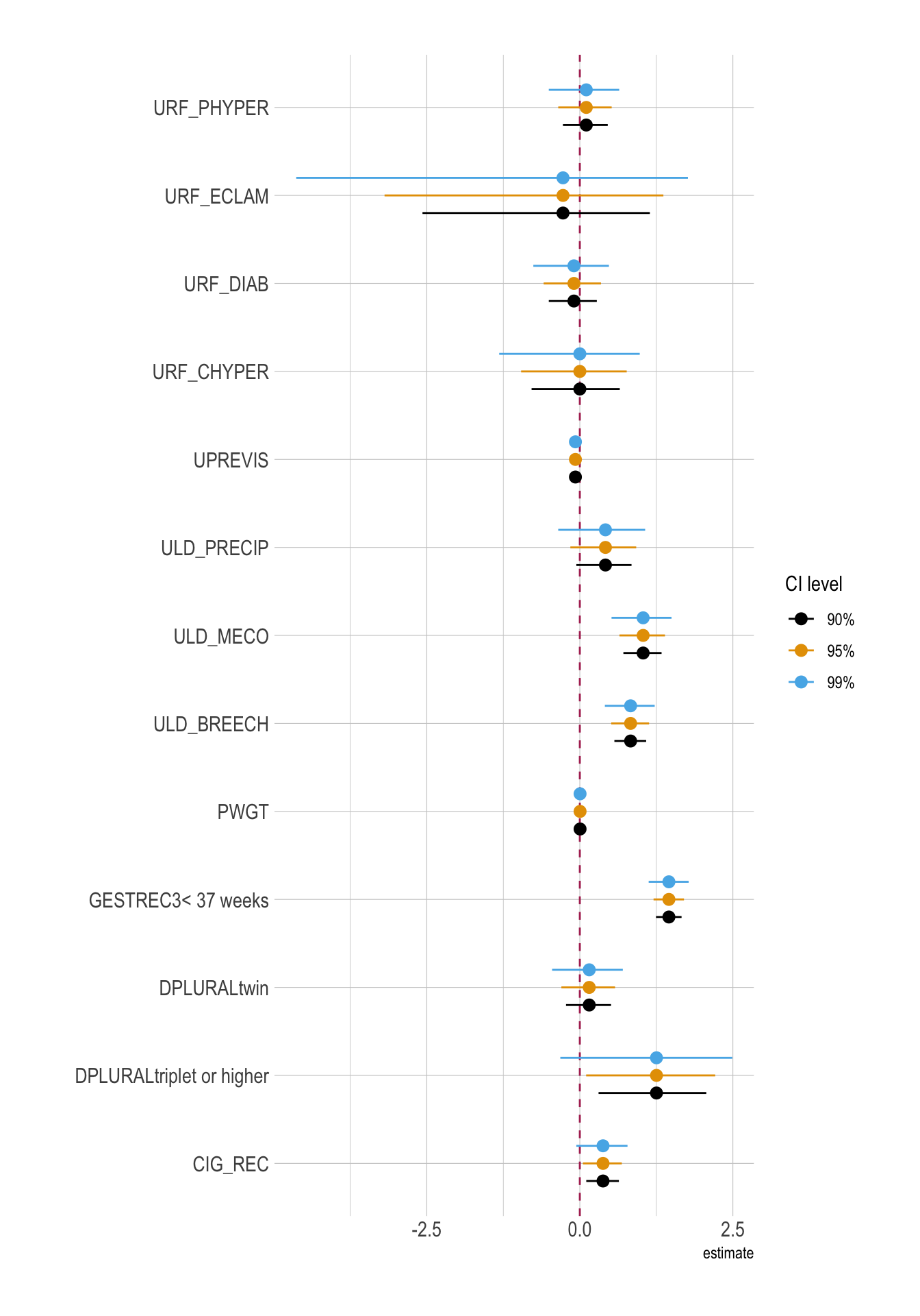
conf.level = 0.99)Coefficient Plots
month_ci <- bind_rows(
  model_betas_90ci |> mutate(ci = "90%"),
  model_betas      |> mutate(ci = "95%"),
  model_betas_99ci |> mutate(ci = "99%")
) |>
  mutate(ci = factor(ci, levels = c("90%", "95%", "99%")))

ggplot(
  data = month_ci |>
    filter(!str_detect(term, "Intercept")),
  aes(
    y = term,
    x = estimate,
    xmin = conf.low,
    xmax = conf.high,
    color = ci
  )
) +
  geom_vline(xintercept = 0, color = "maroon", linetype = 2) +
  geom_pointrange(
    position = position_dodge(width = 0.6)
  ) +
  labs(
    color = "CI level",
    y = ""
) 
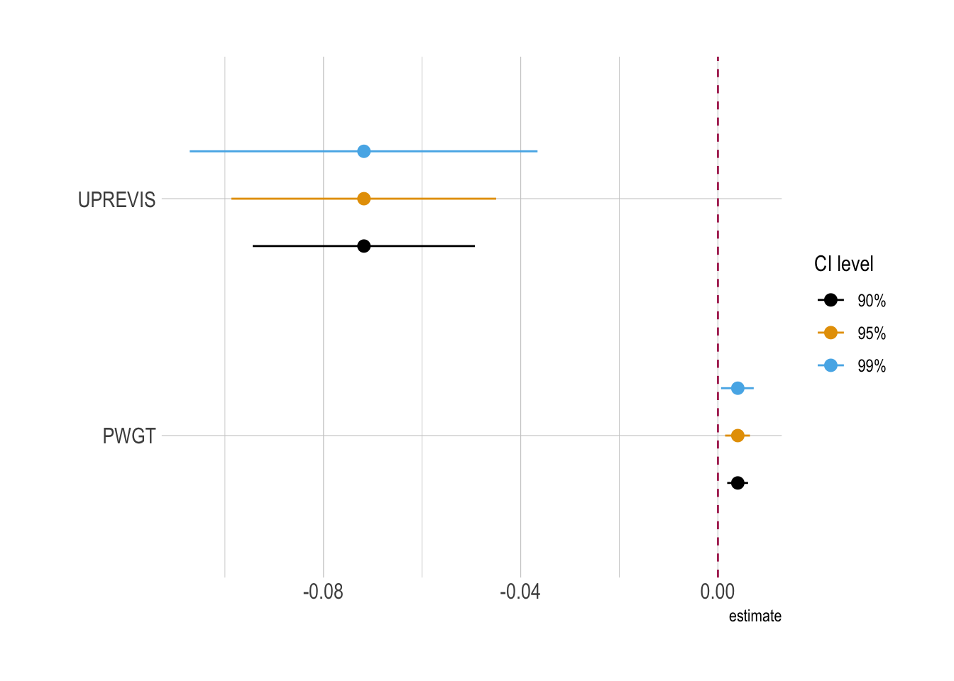
ggplot(
  data = month_ci |>
    filter(term %in% c("UPREVIS", "PWGT")),
  aes(
    y = term,
    x = estimate,
    xmin = conf.low,
    xmax = conf.high,
    color = ci
  )
) +
  geom_vline(xintercept = 0, color = "maroon", linetype = 2) +
  geom_pointrange(
    position = position_dodge(width = 0.6)
  ) +
  labs(
    color = "CI level",
    y = ""
) 
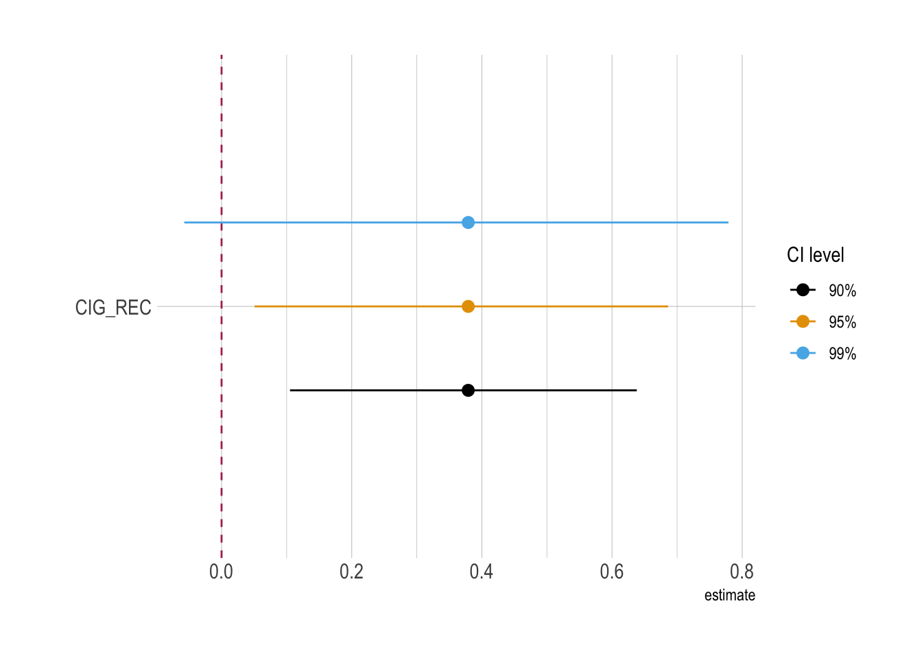
ggplot(
  data = month_ci |>
    filter(term %in% c("CIG_REC")),
  aes(
    y = term,
    x = estimate,
    xmin = conf.low,
    xmax = conf.high,
    color = ci
  )
) +
  geom_vline(xintercept = 0, color = "maroon", linetype = 2) +
  geom_pointrange(
    position = position_dodge(width = 0.6)
  ) +
  labs(
    color = "CI level",
    y = ""
) 
Model Fit (glance())
model |>
  glance() |>
  paged_table()
Marginal Effects (margins())
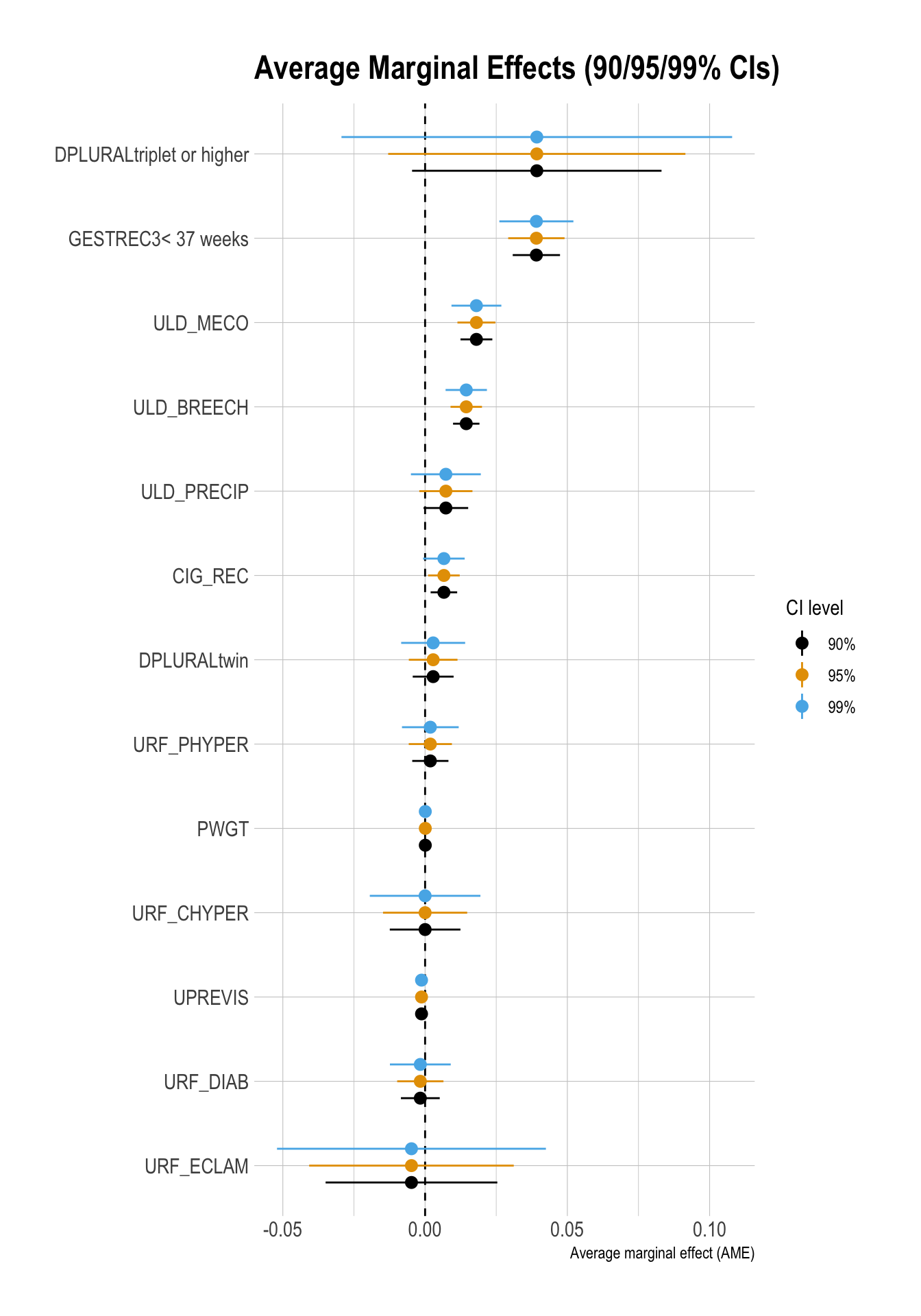
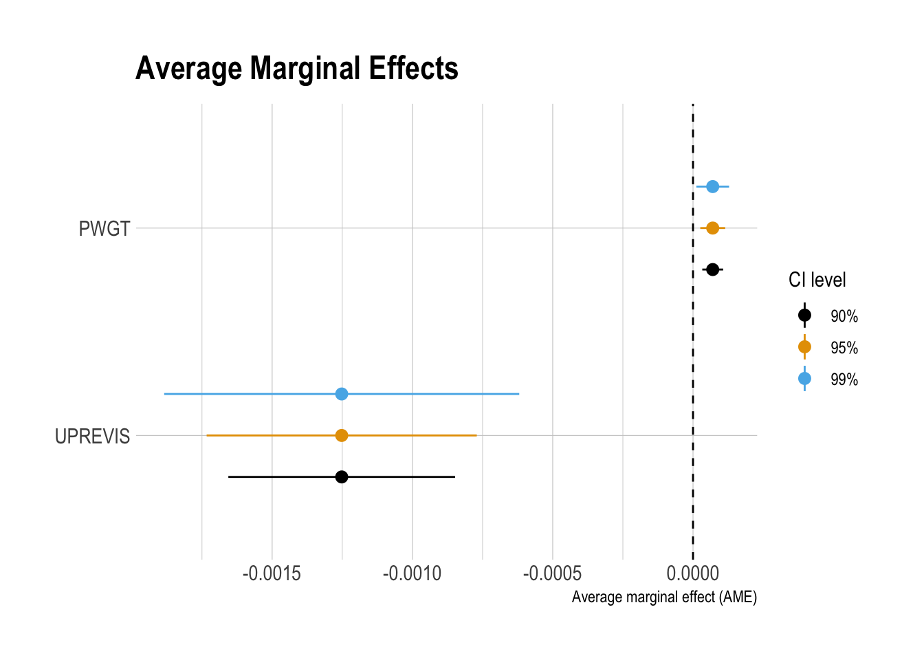
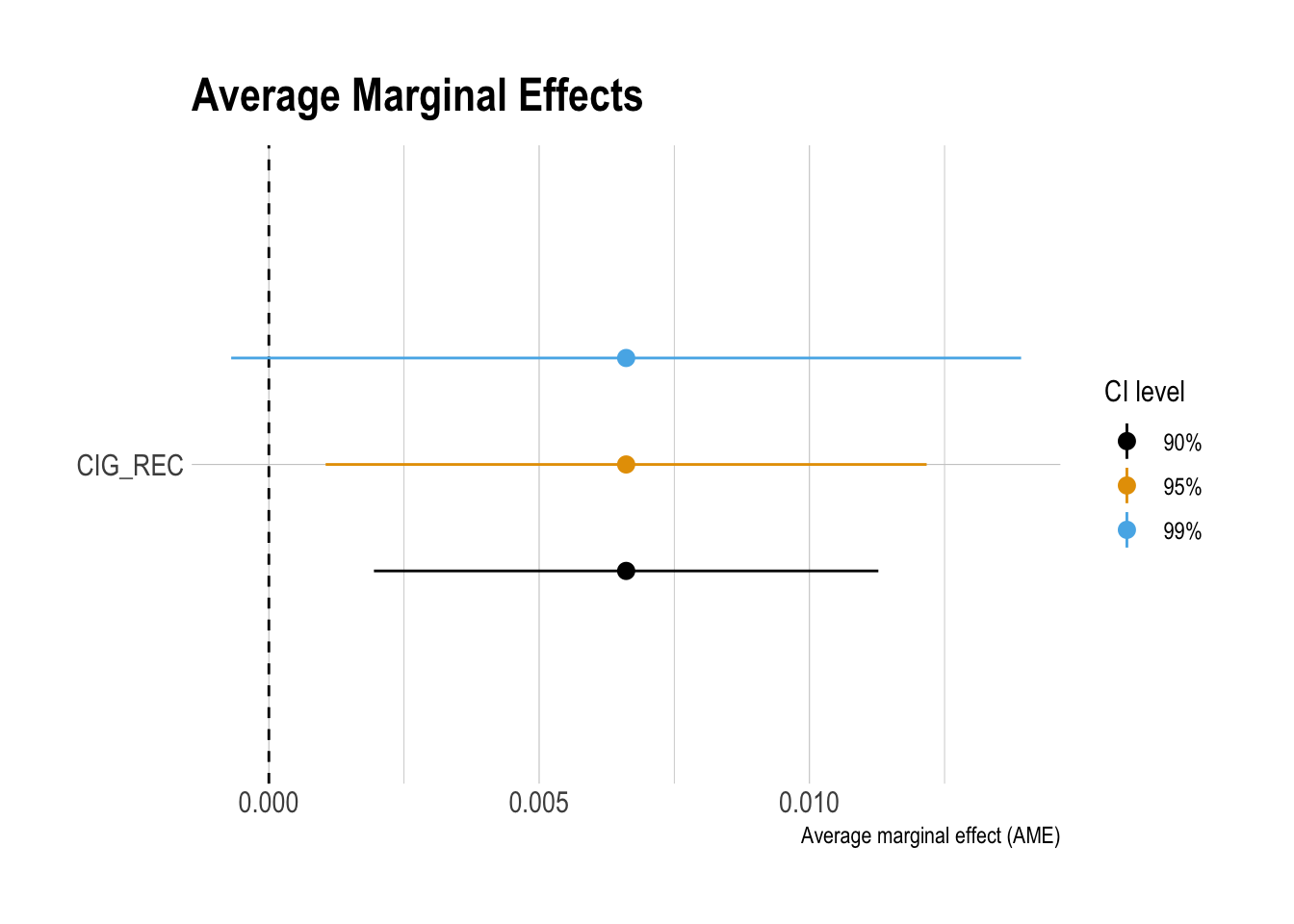
Average Marginal Effects
me <- margins(model)
sum_me <- summary(me)
sum_me
factor AME SE z p lower upper
CIG_REC 0.0066 0.0028 2.3303 0.0198 0.0011 0.0122
DPLURALtriplet or higher 0.0393 0.0266 1.4732 0.1407 -0.0130 0.0915
DPLURALtwin 0.0028 0.0044 0.6494 0.5161 -0.0057 0.0114
GESTREC3< 37 weeks 0.0391 0.0051 7.7424 0.0000 0.0292 0.0490
PWGT 0.0001 0.0000 3.1037 0.0019 0.0000 0.0001
ULD_BREECH 0.0145 0.0028 5.1292 0.0000 0.0089 0.0200
ULD_MECO 0.0180 0.0034 5.3008 0.0000 0.0114 0.0247
ULD_PRECIP 0.0073 0.0048 1.5315 0.1256 -0.0020 0.0166
UPREVIS -0.0013 0.0002 -5.0975 0.0000 -0.0017 -0.0008
URF_CHYPER 0.0000 0.0075 0.0006 0.9995 -0.0148 0.0148
URF_DIAB -0.0017 0.0041 -0.4042 0.6860 -0.0098 0.0065
URF_ECLAM -0.0048 0.0183 -0.2613 0.7939 -0.0407 0.0312
URF_PHYPER 0.0018 0.0039 0.4760 0.6341 -0.0057 0.0094Marginal Effects for Selected Variables
summary(
  margins(model,
          variables = c("PWGT", "UPREVIS", "CIG_REC"))
)
factor AME SE z p lower upper
CIG_REC 0.0066 0.0028 2.3303 0.0198 0.0011 0.0122
PWGT 0.0001 0.0000 3.1037 0.0019 0.0000 0.0001
UPREVIS -0.0013 0.0002 -5.0975 0.0000 -0.0017 -0.0008Interpreting AMEs from margins() (Outcome: atRisk = 1)
AME = average change in \(\Pr(\text{atRisk}=1)\) when the predictor increases by 1 unit
(holding other variables at their observed values, then averaging across the sample).
1) CIG_REC (smoker indicator: 1 = smoker, 0 = non-smoker)
- AME = 0.0066 (p = 0.0198; 95% CI [0.0011, 0.0122])
- Interpretation: on average, changing
CIG_RECfrom 0 → 1 (non-smoker → smoker) increases \(\Pr(\text{atRisk}=1)\) by 0.0066. - In percentage points: \(0.0066 \times 100 = 0.66\) → +0.66 pp (95% CI: +0.11 to +1.22 pp)
Plain-English: babies of smokers have an estimated 0.66 percentage point higher probability of being atRisk, on average, compared to babies of non-smokers (holding other covariates constant on average).
2) PWGT = Prepregnancy weight (numeric)
- AME = 0.0001 (p = 0.0019; 95% CI [0.0000, 0.0001])
- Interpretation: a 1-unit increase in prepregnancy weight changes \(\Pr(\text{atRisk}=1)\) by +0.0001 on average.
- In percentage points: +0.01 pp per 1 unit
Rescale (PWGT is in pounds):
- +10 lb: \(10 \times 0.0001 = 0.0010\) → +0.10 pp
- +50 lb: \(50 \times 0.0001 = 0.0050\) → +0.50 pp
- +100 lb: \(100 \times 0.0001 = 0.0100\) → +1.00 pp
3) UPREVIS = Prenatal visits (integer)
- AME = -0.0013 (p < 0.001; 95% CI [-0.0017, -0.0008])
- Interpretation: each additional prenatal visit changes \(\Pr(\text{atRisk}=1)\) by −0.0013 on average.
- In percentage points: \(-0.0013 \times 100 = -0.13\) → −0.13 pp per visit
Rescale: - +5 visits: −0.65 pp - +10 visits: −1.30 pp - +15 visits: −1.95 pp
## Marginal Effect Plots
df_ame <- sum_me |>
  as_tibble() |>
  rename(
    term = factor,
    ame  = AME,
    se   = SE
  )

# Pair each level with the correct z (NOT a Cartesian product)
ci_levels <- tibble(
  level = c("90%", "95%", "99%"),
  zcrit = c(1.645, 1.96, 2.576)
)

df_ame_ci <- df_ame |>
  tidyr::crossing(level = ci_levels$level) |>
  left_join(ci_levels, by = "level") |>
  mutate(
    conf.low  = ame - zcrit * se,
    conf.high = ame + zcrit * se
  )

ggplot(df_ame_ci,
       aes(x = fct_reorder(term, ame), y = ame)) +
  geom_hline(yintercept = 0, linetype = "dashed") +
  geom_pointrange(
    aes(ymin = conf.low, ymax = conf.high, color = level),
    position = position_dodge(width = 0.6)
  ) +
  coord_flip() +
  labs(
    x = NULL,
    y = "Average marginal effect (AME)",
    color = "CI level",
    title = "Average Marginal Effects (90/95/99% CIs)"
  )
ggplot(data = df_ame_ci |>
         filter(term %in% c("PWGT", "UPREVIS") ),
       aes(x = fct_reorder(term, ame),
           y = ame)) +
  geom_hline(yintercept = 0,
             linetype = "dashed") +
  geom_pointrange(
    aes(ymin = conf.low,
        ymax = conf.high,
        color = level),
    position = position_dodge(width = 0.6)
  ) +
  coord_flip() +
  labs(
    x = NULL,
    y = "Average marginal effect (AME)",
    color = "CI level",
    title = "Average Marginal Effects"
  )
ggplot(data = df_ame_ci |>
         filter(term %in% c("CIG_REC") ),
       aes(x = fct_reorder(term, ame),
           y = ame)) +
  geom_hline(yintercept = 0,
             linetype = "dashed") +
  geom_pointrange(
    aes(ymin = conf.low,
        ymax = conf.high,
        color = level),
    position = position_dodge(width = 0.6)
  ) +
  coord_flip() +
  labs(
    x = NULL,
    y = "Average marginal effect (AME)",
    color = "CI level",
    title = "Average Marginal Effects"
  )
Classification
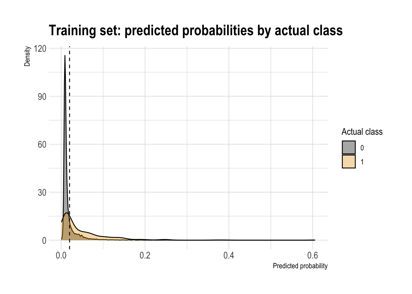
Double density plot (threshold intuition)
threshold <- 0.02

# dtest <- dtest |>
#   mutate(.fitted = predict(model,
#                            newdata = dtest,
#                            type = "response"))

model |>
  augment(type.predict = "response") |>
  ggplot(aes(x = .fitted,
             fill = factor(atRisk))) +
  geom_density(alpha = 0.35) +
  geom_vline(xintercept = threshold, linetype = "dashed") +
  labs(
    x = "Predicted probability",
    y = "Density",
    fill = "Actual class",
    title = "Training set: predicted probabilities by actual class"
  )
Confusion Matrix
threshold <- 0.02

df_cm <- model |>
  augment(newdata = dtest,
          type.predict = "response") |>
  mutate(
    actual = factor(atRisk,
                    levels = c(0, 1),
                    labels = c("not at-risk", "at-risk")),
    pred   = factor(if_else(.fitted > threshold, 1, 0),
                    levels = c(0, 1),
                    labels = c("not at-risk", "at-risk"))
  )

conf_mat <- table(truth = df_cm$actual,
                  prediction = df_cm$pred)
conf_mat
prediction
truth not at-risk at-risk
not at-risk 6107 1480
at-risk 69 73# data.frame of confusion matrix
cm_counts <- df_cm |>
group_by(actual, pred) |>
summarize(n = n()) |>
ungroup() |>
pivot_wider(names_from = pred,
values_from = n,
values_fill = 0) |>
rename(`truth / prediction` = actual)
cm_counts# A tibble: 2 × 3
`truth / prediction` `not at-risk` `at-risk`
<fct> <int> <int>
1 not at-risk 6107 1480
2 at-risk 69 73Performance Metrics (from conf_mat)
base_rate   <- mean(dtest$atRisk)

accuracy <- (conf_mat[1,1] + conf_mat[2,2]) / sum(conf_mat)
precision <- conf_mat[2,2] / sum(conf_mat[,2])
recall <- conf_mat[2,2] / sum(conf_mat[2,])
specificity <- conf_mat[1,1] / sum(conf_mat[1,])
enrichment <- precision / base_rate


df_class_metric <-
  data.frame(
    metric = c("Base rate",
               "Accuracy",
               "Precision",
               "Recall",
               "Specificity",
               "Enrichment"),
    value  = c(base_rate,
               accuracy,
               precision,
               recall,
               specificity,
               enrichment)
    )

df_class_metric |>
  mutate(value = round(value, 4)) |>
  rmarkdown::paged_table()
Performance Metrics (from df_cm)
Code
# Pull counts from df_cm (no matrix())
TN <- sum(df_cm$actual == "not at-risk" & df_cm$pred == "not at-risk")
TP <- sum(df_cm$actual == "at-risk" & df_cm$pred == "at-risk")
FN <- sum(df_cm$actual == "at-risk" & df_cm$pred == "not at-risk")
FP <- sum(df_cm$actual == "not at-risk" & df_cm$pred == "at-risk")

accuracy    <- (TP + TN) / (TP + FP + FN + TN)
precision   <- TP / (TP + FP)
recall      <- TP / (TP + FN)         # sensitivity
specificity <- TN / (TN + FP)

base_rate   <- mean(dtest$atRisk)
enrichment  <- precision / base_rate

df_class_metric <-
  data.frame(
    metric = c("Base rate",
               "Accuracy",
               "Precision",
               "Recall",
               "Specificity",
               "Enrichment"),
    value  = c(base_rate,
               accuracy,
               precision,
               recall,
               specificity,
               enrichment)
    )

df_class_metric |>
  mutate(value = round(value, 4)) |>
  rmarkdown::paged_table()
Precision/Recall/Enrichment Curves over Thresholds (using WVPlots package)
plt <- PRTPlot(df_cm,
               ".fitted", "atRisk", 1,
               plotvars = c("enrichment", "precision", "recall", "specificity", "false_positive_rate"),
               thresholdrange = c(0,.1),
               title = "Enrichment vs. recall with threshold for natality model")

plt +
  geom_vline(xintercept = threshold,
             color="maroon",
             linetype = 2)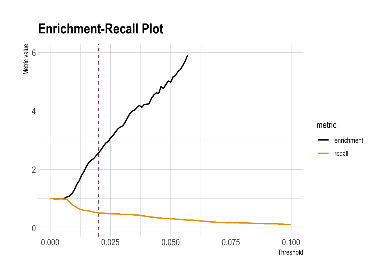
ROC and AUC (using WVPlots and pROC packages)
roc <- ROCPlot(df_cm,
               xvar = '.fitted',
               truthVar = 'atRisk',
               truthTarget = 1,
               title = 'Classifier performance')

# ROC with vertical line
roc +
  geom_vline(xintercept = 1 - specificity,
             color="maroon", linetype = 2)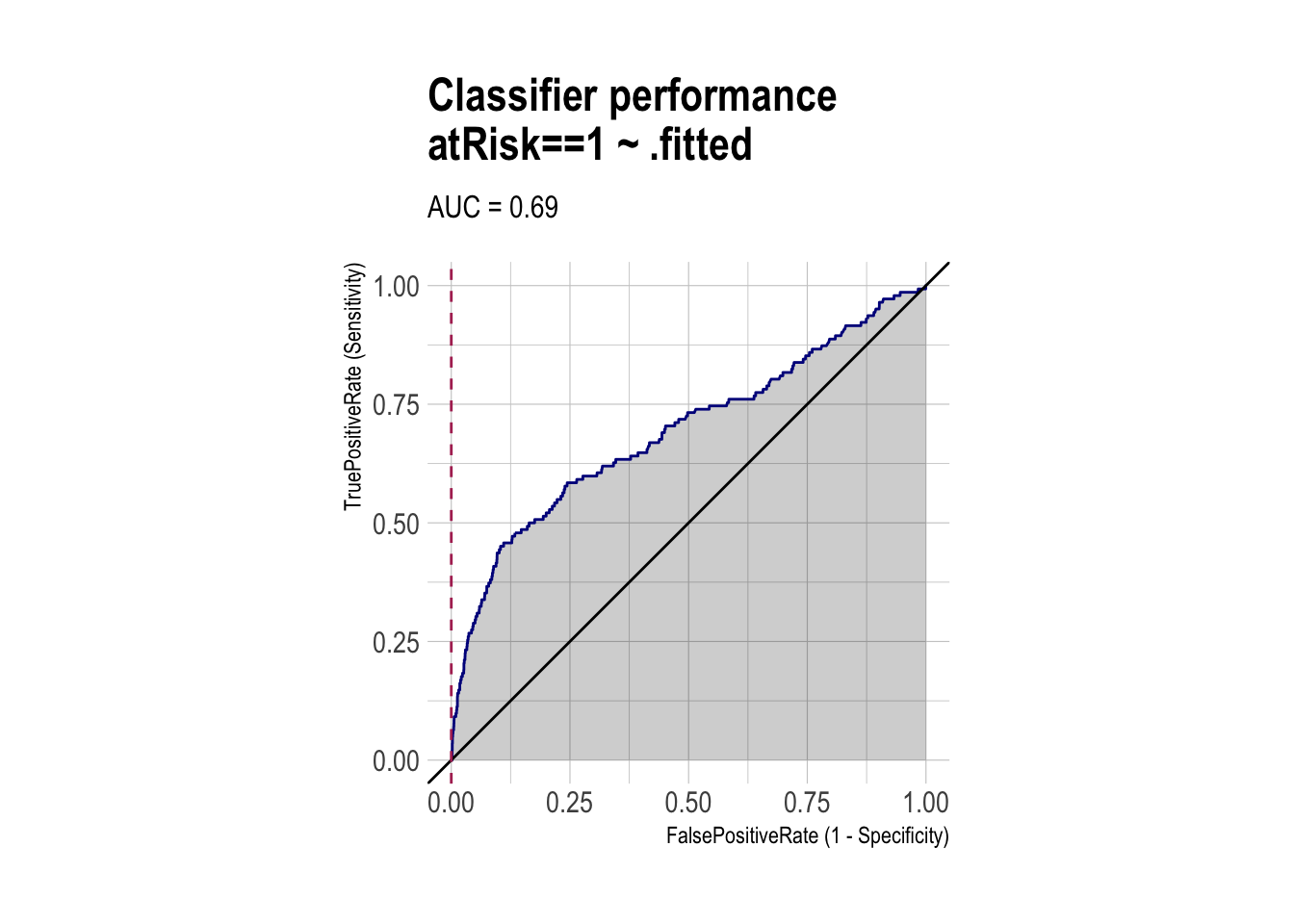
# AUC
# pROC::roc(BINARY_OUTCOME, PREDICTED_PROBABILITY)
roc_obj <- roc(df_cm$atRisk, df_cm$.fitted)
auc(roc_obj)
Area under the curve: 0.6914Classifier Performance Can Shift with Base Rates
Performance of Classifier (NY → MA thought experiment)
- Suppose you trained a classifier on NY hospital data with acceptable precision/recall.
- Now you apply the same classifier to MA hospitals.
- Will it perform as well?
- Even if the relationship between features and risk is similar, the base rate (share of at-risk babies) in MA may differ.
- This can change precision a lot, even when recall stays similar.
Create MA-like test sets with different at-risk rates (R)
set.seed(23464)

# Take 1,000 observations out of the test set (to "swap" base rates)
sample_indices <- sample(seq_len(nrow(dtest)), size = 1000, replace = FALSE)

separated <- dtest[sample_indices, ]
dtest_NY  <- dtest[-sample_indices, ]   # treat as "NY hospitals"

# Split the separated chunk into at-risk vs not-at-risk
at_risk_sample     <- separated |> filter(atRisk == 1)
not_at_risk_sample <- separated |> filter(atRisk == 0)

# MA test sets with different prevalence (base rates)
dtest_MA_moreRisk <- bind_rows(dtest_NY, at_risk_sample)       # add back only at-risk cases
dtest_MA_lessRisk <- bind_rows(dtest_NY, not_at_risk_sample)   # add back only not-at-risk cases

# Verify sizes
tibble(
  dataset = c("Original test", "Separated", "NY hospitals",
              "MA (more risk)", "MA (less risk)"),
  n = c(nrow(dtest), nrow(separated), nrow(dtest_NY),
        nrow(dtest_MA_moreRisk), nrow(dtest_MA_lessRisk)),
  at_risk_rate = c(mean(dtest$atRisk),
                   mean(separated$atRisk),
                   mean(dtest_NY$atRisk),
                   mean(dtest_MA_moreRisk$atRisk),
                   mean(dtest_MA_lessRisk$atRisk))
)
# A tibble: 5 × 3
dataset n at_risk_rate
<chr> <int> <dbl>
1 Original test 7729 0.0184
2 Separated 1000 0.0320
3 NY hospitals 6729 0.0163
4 MA (more risk) 6761 0.0210
5 MA (less risk) 7697 0.0143NY test data
df_cm_NY <- model |>
  augment(newdata = dtest_NY,
          type.predict = "response") |>
  mutate(
    actual = factor(atRisk,
                    levels = c(0, 1),
                    labels = c("not at-risk", "at-risk")),
    pred   = factor(if_else(.fitted > threshold, 1, 0),
                    levels = c(0, 1),
                    labels = c("not at-risk", "at-risk"))
  )


conf_mat_NY <- table(truth = df_cm_NY$actual,
                           prediction = df_cm_NY$pred)
conf_mat_NY
prediction
truth not at-risk at-risk
not at-risk 5318 1301
at-risk 54 56base_rate <- mean(dtest_NY$atRisk)
accuracy <- (conf_mat_NY[1,1] + conf_mat_NY[2,2]) / sum(conf_mat_NY)
precision <- conf_mat_NY[2,2] / sum(conf_mat_NY[,2])
recall <- conf_mat_NY[2,2] / sum(conf_mat_NY[2,])
specificity <- conf_mat_NY[1,1] / sum(conf_mat_NY[1,])
enrichment <- precision / base_rate
df_class_metric_NY <-
data.frame(
metric = c("Base rate",
"Accuracy",
"Precision",
"Recall",
"Specificity",
"Enrichment"),
value = c(base_rate,
accuracy,
precision,
recall,
specificity,
enrichment)
)Evaluate the same classifier on each test set (fixed threshold)
df_cm_MA_moreRisk <- model |>
  augment(newdata = dtest_MA_moreRisk,
          type.predict = "response") |>
  mutate(
    actual = factor(atRisk,
                    levels = c(0, 1),
                    labels = c("not at-risk", "at-risk")),
    pred   = factor(if_else(.fitted > threshold, 1, 0),
                    levels = c(0, 1),
                    labels = c("not at-risk", "at-risk"))
  )


conf_mat_moreRisk <- table(truth = df_cm_MA_moreRisk$actual,
                           prediction = df_cm_MA_moreRisk$pred)
conf_mat_moreRisk
prediction
truth not at-risk at-risk
not at-risk 5318 1301
at-risk 69 73base_rate <- mean(dtest_MA_moreRisk$atRisk)
accuracy <- (conf_mat_moreRisk[1,1] + conf_mat_moreRisk[2,2]) / sum(conf_mat_moreRisk)
precision <- conf_mat_moreRisk[2,2] / sum(conf_mat_moreRisk[,2])
recall <- conf_mat_moreRisk[2,2] / sum(conf_mat_moreRisk[2,])
specificity <- conf_mat_moreRisk[1,1] / sum(conf_mat_moreRisk[1,])
enrichment <- precision / base_rate
df_class_metric_MA_moreRisk <-
data.frame(
metric = c("Base rate",
"Accuracy",
"Precision",
"Recall",
"Specificity",
"Enrichment"),
value = c(base_rate,
accuracy,
precision,
recall,
specificity,
enrichment)
)df_cm_MA_lessRisk <- model |>
augment(newdata = dtest_MA_lessRisk,
type.predict = "response") |>
mutate(
actual = factor(atRisk,
levels = c(0, 1),
labels = c("not at-risk", "at-risk")),
pred = factor(if_else(.fitted > threshold, 1, 0),
levels = c(0, 1),
labels = c("not at-risk", "at-risk"))
)
conf_mat_lessRisk <- table(truth = df_cm_MA_lessRisk$actual,
prediction = df_cm_MA_lessRisk$pred)
conf_mat_lessRisk prediction
truth not at-risk at-risk
not at-risk 6107 1480
at-risk 54 56base_rate <- mean(dtest_MA_lessRisk$atRisk)
accuracy <- (conf_mat_lessRisk[1,1] + conf_mat_lessRisk[2,2]) / sum(conf_mat_lessRisk)
precision <- conf_mat_lessRisk[2,2] / sum(conf_mat_lessRisk[,2])
recall <- conf_mat_lessRisk[2,2] / sum(conf_mat_lessRisk[2,])
specificity <- conf_mat_lessRisk[1,1] / sum(conf_mat_lessRisk[1,])
enrichment <- precision / base_rate
df_class_metric_MA_lessRisk <-
data.frame(
metric = c("Base rate",
"Accuracy",
"Precision",
"Recall",
"Specificity",
"Enrichment"),
value = c(base_rate,
accuracy,
precision,
recall,
specificity,
enrichment)
)df_class_metric_NY |>
rmarkdown::paged_table()df_class_metric_MA_moreRisk |>
rmarkdown::paged_table()df_class_metric_MA_lessRisk |>
rmarkdown::paged_table()df_class_metric_all <- df_class_metric_NY |>
left_join(
df_class_metric_MA_moreRisk |>
rename(value_MA_moreRisk = value)
) |>
left_join(
df_class_metric_MA_lessRisk |>
rename(value_MA_lessRisk = value)
) |>
mutate(
pct_chg_MA_moreRisk = 100 * (value_MA_moreRisk - value)/value,
pct_chg_MA_lessRisk = 100 * (value_MA_lessRisk - value)/value
) |>
mutate(
value = round(value, 4),
value_MA_moreRisk = round(value_MA_moreRisk, 4),
value_MA_lessRisk = round(value_MA_lessRisk, 4),
pct_chg_MA_moreRisk = round(pct_chg_MA_moreRisk, 2),
pct_chg_MA_lessRisk = round(pct_chg_MA_lessRisk, 2),
)
df_class_metric_all |>
select(metric, starts_with("value")) |>
rmarkdown::paged_table()df_class_metric_all |>
select(metric, starts_with("pct")) |>
rmarkdown::paged_table()Why Precision Changes a Lot When the Base Rate Changes (Intuition)
In our hospital “at-risk” classifier, the base rate (prevalence) is tiny:
- Only about 1–2% of hospitals are truly at-risk.
But our classifier has a fairly large false positive rate (FPR):
- About 20% of not at-risk hospitals get flagged as at-risk.
That combination is the whole story.
1) Recall vs Precision: what they “condition on”
Recall (Sensitivity / TPR) asks:
“Among hospitals that are truly at-risk, how many did we catch?”
\[ \text{Recall} = \frac{TP}{TP + FN} \]
This focuses only on the true at-risk group, so it is not directly affected by how many at-risk hospitals exist overall.
Precision (PPV) asks:
“Among hospitals predicted as at-risk, how many are truly at-risk?”
\[ \text{Precision} = \frac{TP}{TP + FP} \]
This depends heavily on the number of false alarms (\(FP\)).
When the base rate is low, even a moderate \(FPR\) creates many false alarms because there are so many more not at-risk hospitals.
2) Intuition
- Recall stays similar because it measures performance within the true at-risk group: \(\frac{TP}{TP+FN}\).
- Precision drops when the base rate drops because the false alarms (\(FP\)) come from the huge not at-risk group and can overwhelm the few true positives.
3) A “100,000 hospitals” thought experiment
Assume the classifier behavior stays the same across places:
- \(\text{TPR} \approx 0.51\)
- \(\text{FPR} \approx 0.195\)
Case A: Higher base rate (2% at-risk)
Out of \(100{,}000\) hospitals:
- Truly at-risk: \(2\% \Rightarrow 2{,}000\)
- Not at-risk: \(98{,}000\)
Apply the classifier:
- True positives: \(TP \approx 0.51 \times 2{,}000 = 1{,}020\)
- False positives: \(FP \approx 0.195 \times 98{,}000 = 19{,}110\)
Predicted “at-risk”: \[ TP + FP \approx 1{,}020 + 19{,}110 = 20{,}130 \]
Precision: \[ \text{Precision} \approx \frac{1{,}020}{20{,}130} \approx 0.051 \]
Recall: \[ \text{Recall} \approx 0.51 \]
Case B: Lower base rate (1.4% at-risk)
Out of \(100{,}000\) hospitals:
- Truly at-risk: \(1.4\% \Rightarrow 1{,}400\)
- Not at-risk: \(98{,}600\)
Apply the classifier:
- True positives: \(TP \approx 0.51 \times 1{,}400 = 714\)
- False positives: \(FP \approx 0.195 \times 98{,}600 = 19{,}227\)
Predicted “at-risk”: \[ TP + FP \approx 714 + 19{,}227 = 19{,}941 \]
Precision: \[ \text{Precision} \approx \frac{714}{19{,}941} \approx 0.036 \]
Recall: \[ \text{Recall} \approx 0.51 \]