library(tidyverse)
library(broom)
library(stargazer)
library(skimr)
library(DT)Linear Regression II
Orange Juice Data
R packages
Read_statusing a CSV File
df <- read_csv("https://bcdanl.github.io/data/dominick_oj_feat.csv")Variable description
| Variable | Description |
|---|---|
sales |
Quantity of OJ cartons sold |
price |
Price of OJ |
brand |
Brand of OJ |
ad_status |
ad_statusvertisement status |
Continuous variables
salesprice
Categorical variables
brandad_status
Exploratory Data Analysis
skim(df)| Name | df |
| Number of rows | 28947 |
| Number of columns | 4 |
| _______________________ | |
| Column type frequency: | |
| character | 2 |
| numeric | 2 |
| ________________________ | |
| Group variables | None |
Variable type: character
| skim_variable | n_missing | complete_rate | min | max | empty | n_unique | whitespace |
|---|---|---|---|---|---|---|---|
| brand | 0 | 1 | 9 | 11 | 0 | 3 | 0 |
| ad_status | 0 | 1 | 2 | 5 | 0 | 2 | 0 |
Variable type: numeric
| skim_variable | n_missing | complete_rate | mean | sd | p0 | p25 | p50 | p75 | p100 | hist |
|---|---|---|---|---|---|---|---|---|---|---|
| sales | 0 | 1 | 17312.21 | 27477.66 | 64.00 | 4864.00 | 8384.00 | 17408.00 | 716416.00 | ▇▁▁▁▁ |
| price | 0 | 1 | 2.28 | 0.65 | 0.52 | 1.79 | 2.17 | 2.73 | 3.87 | ▁▆▇▅▂ |
Distribution
df |>
  ggplot(aes(x = price, color = brand)) +
  geom_freqpoly()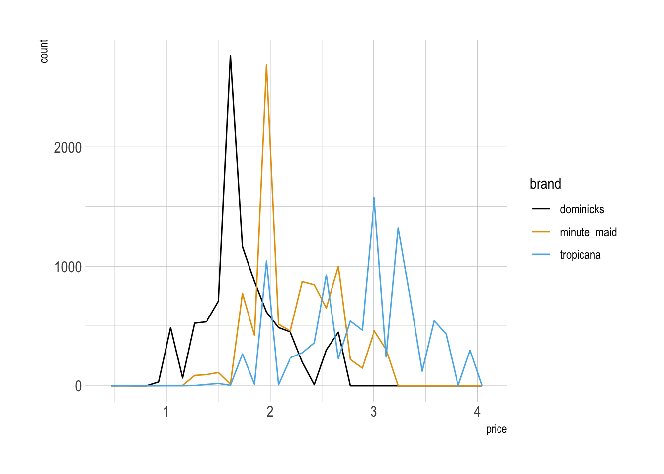
Categorical Variables
df |>
  count(brand, ad_status) |>
  ggplot() +
  geom_col(aes(x = ad_status, y = n,
               fill = brand),
           position = "fill")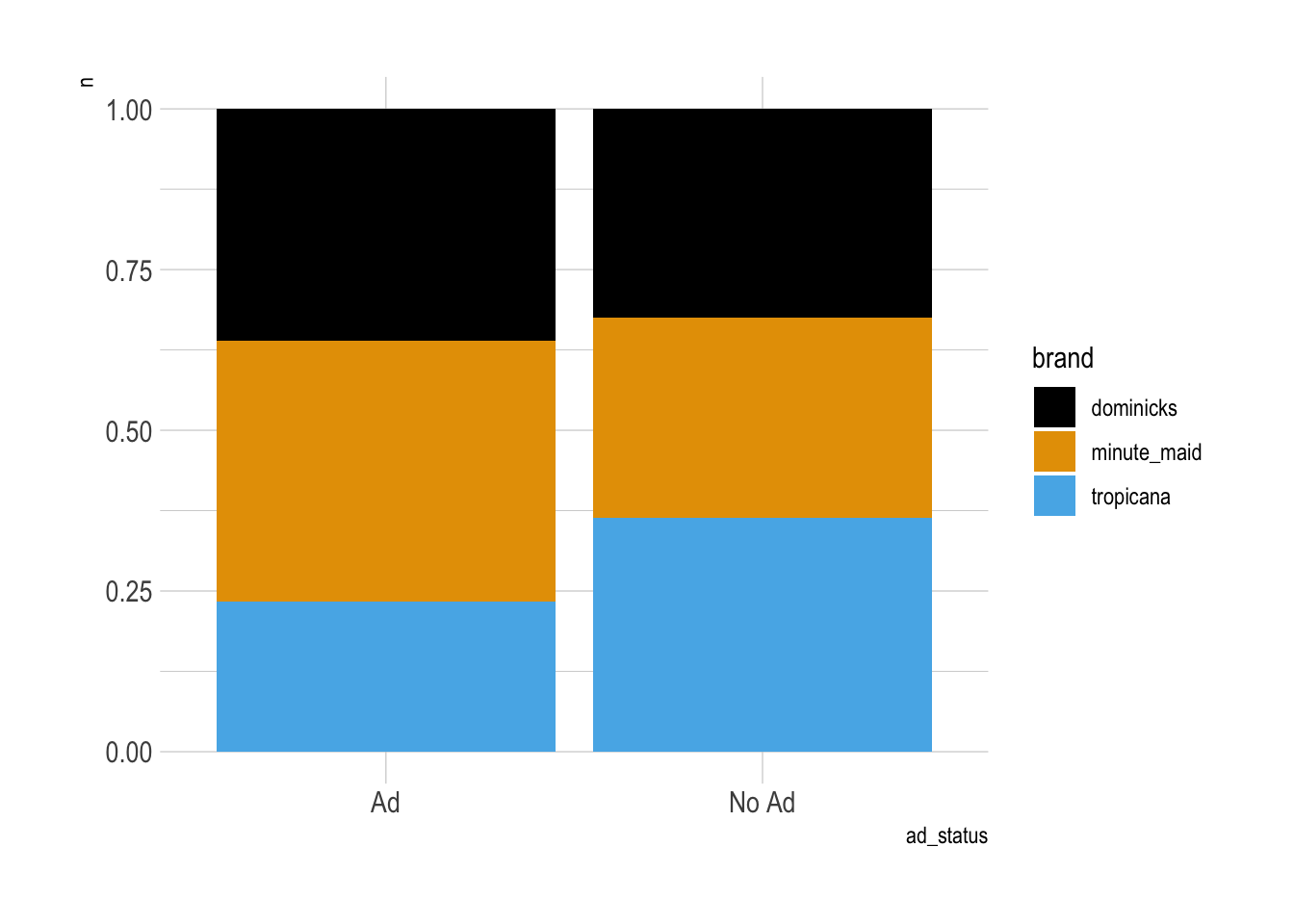
Data Preparation
df <- df |>
  mutate(ad_status = factor(ad_status),
         ad_status = fct_relevel(ad_status, "No Ad")
         )
Training and Test Data
set.seed(1)

df <- df |>
  mutate(rnd = runif(n()))

dtrain <- df |>
  filter(rnd > 0.3)

dtest <- df |>
  filter(rnd <= 0.3)

nrow(dtrain) / nrow(df)
[1] 0.6971707Models
Model 1
\[ \begin{align} \log(\texttt{sales}_{\texttt{i}}) \,=\, &\quad\;\; b_{\texttt{intercept}} \\ &\,+\,b_{\,\texttt{mm}}\,\texttt{brand}_{\,\texttt{mm}, \texttt{i}} \,+\, b_{\,\texttt{tr}}\,\texttt{brand}_{\,\texttt{tr}, \texttt{i}}\\ &\,+\, b_{\texttt{price}}\,\log(\texttt{price}_{\texttt{i}}) \,+\, e_{\texttt{i}} \end{align} \]
Model 2
\[ \begin{align} \log(\texttt{sales}_{\texttt{i}}) \,=\,&\;\; \quad b_{\texttt{intercept}} \,+\, \color{Green}{b_{\,\texttt{mm}}\,\texttt{brand}_{\,\texttt{mm}, \texttt{i}}} \,+\, \color{Blue}{b_{\,\texttt{tr}}\,\texttt{brand}_{\,\texttt{tr}, \texttt{i}}}\\ &\,+\, b_{\texttt{price}}\,\log(\texttt{price}_{\texttt{i}}) \\ &\, +\, b_{\texttt{price*mm}}\,\log(\texttt{price}_{\texttt{i}})\,\times\,\color{Green} {\texttt{brand}_{\,\texttt{mm}, \texttt{i}}} \\ &\,+\, b_{\texttt{price*tr}}\,\log(\texttt{price}_{\texttt{i}})\,\times\,\color{Blue} {\texttt{brand}_{\,\texttt{tr}, \texttt{i}}} \,+\, e_{\texttt{i}} \end{align} \]
Model 3
\[ \begin{align} \log(\texttt{sales}_{\texttt{i}}) \,=\,\quad\;\;& b_{\texttt{intercept}} \,+\, \color{Green}{b_{\,\texttt{mm}}\,\texttt{brand}_{\,\texttt{mm}, \texttt{i}}} \,+\, \color{Blue}{b_{\,\texttt{tr}}\,\texttt{brand}_{\,\texttt{tr}, \texttt{i}}} \\ &\,+\; b_{\,\texttt{ad}}\,\color{Orange}{\texttt{ad}_{\,\texttt{i}}} \qquad\qquad\qquad\qquad\quad \\ &\,+\, b_{\texttt{mm*ad}}\,\color{Green} {\texttt{brand}_{\,\texttt{mm}, \texttt{i}}}\,\times\, \color{Orange}{\texttt{ad}_{\,\texttt{i}}}\,+\, b_{\texttt{tr*ad}}\,\color{Blue} {\texttt{brand}_{\,\texttt{tr}, \texttt{i}}}\,\times\, \color{Orange}{\texttt{ad}_{\,\texttt{i}}} \\ &\,+\; b_{\texttt{price}}\,\log(\texttt{price}_{\texttt{i}}) \qquad\qquad\qquad\;\;\;\;\, \\ &\,+\, b_{\texttt{price*mm}}\,\log(\texttt{price}_{\texttt{i}})\,\times\,\color{Green} {\texttt{brand}_{\,\texttt{mm}, \texttt{i}}}\qquad\qquad\qquad\;\, \\ &\,+\, b_{\texttt{price*tr}}\,\log(\texttt{price}_{\texttt{i}})\,\times\,\color{Blue} {\texttt{brand}_{\,\texttt{tr}, \texttt{i}}}\qquad\qquad\qquad\;\, \\ & \,+\, b_{\texttt{price*ad}}\,\log(\texttt{price}_{\texttt{i}})\,\times\,\color{Orange}{\texttt{ad}_{\,\texttt{i}}}\qquad\qquad\qquad\;\;\, \\ &\,+\, b_{\texttt{price*mm*ad}}\,\log(\texttt{price}_{\texttt{i}}) \,\times\,\,\color{Green} {\texttt{brand}_{\,\texttt{mm}, \texttt{i}}}\,\times\, \color{Orange}{\texttt{ad}_{\,\texttt{i}}} \\ &\,+\, b_{\texttt{price*tr*ad}}\,\log(\texttt{price}_{\texttt{i}}) \,\times\,\,\color{Blue} {\texttt{brand}_{\,\texttt{tr}, \texttt{i}}}\,\times\, \color{Orange}{\texttt{ad}_{\,\texttt{i}}} \,+\, e_{\texttt{i}} \end{align} \]
Training the Models
m1 <- lm(log(sales) ~ brand + log(price),
         data = dtrain)
m2 <- lm(log(sales) ~ brand * log(price),
         data = dtrain)
m3 <- lm(log(sales) ~ brand * ad_status * log(price),
         data = dtrain)
Regression Table with stargazer()
stargazer(m1, m2, m3,
type = "html")| Dependent variable: | |||
| log(sales) | |||
| (1) | (2) | (3) | |
| brandminute_maid | 0.868*** | 0.908*** | 0.027 |
| (0.015) | (0.050) | (0.056) | |
| brandtropicana | 1.527*** | 0.918*** | 0.696*** |
| (0.019) | (0.055) | (0.060) | |
| ad_statusAd | 1.091*** | ||
| (0.045) | |||
| log(price) | -3.149*** | -3.396*** | -2.795*** |
| (0.027) | (0.043) | (0.046) | |
| brandminute_maid:ad_statusAd | 1.200*** | ||
| (0.097) | |||
| brandtropicana:ad_statusAd | 0.753*** | ||
| (0.118) | |||
| brandminute_maid:log(price) | 0.032 | 0.806*** | |
| (0.068) | (0.074) | ||
| brandtropicana:log(price) | 0.710*** | 0.756*** | |
| (0.064) | (0.068) | ||
| ad_statusAd:log(price) | -0.511*** | ||
| (0.087) | |||
| brandminute_maid:ad_statusAd:log(price) | -1.099*** | ||
| (0.144) | |||
| brandtropicana:ad_statusAd:log(price) | -0.924*** | ||
| (0.149) | |||
| Constant | 10.837*** | 10.967*** | 10.418*** |
| (0.017) | (0.025) | (0.028) | |
| Observations | 20,181 | 20,181 | 20,181 |
| R2 | 0.399 | 0.403 | 0.537 |
| Adjusted R2 | 0.399 | 0.403 | 0.537 |
| Residual Std. Error | 0.795 (df = 20177) | 0.792 (df = 20175) | 0.697 (df = 20169) |
| F Statistic | 4,463.077*** (df = 3; 20177) | 2,726.510*** (df = 5; 20175) | 2,128.289*** (df = 11; 20169) |
| Note: | p<0.1; p<0.05; p<0.01 | ||
Beta Estimates with tidy()
m1_betas <- tidy(m1, conf.int = T)
m2_betas <- tidy(m2, conf.int = T)
m3_betas <- tidy(m3, conf.int = T)
Prediction with predict()
dtest <- dtest |>
  mutate(
    pred_1 = predict(m1, newdata = dtest),
    pred_2 = predict(m2, newdata = dtest),
    pred_3 = predict(m3, newdata = dtest)
  )
Prediction with augment()
m1_pred_train <- augment(m1)
m1_pred_test <- augment(m1, newdata = dtest)
m2_pred_train <- augment(m2)
m2_pred_test <- augment(m2, newdata = dtest)
m3_pred_train <- augment(m3)
m3_pred_test <- augment(m3, newdata = dtest)
Various Model Statistics with glance()
m1_r2 <- glance(m1)
m2_r2 <- glance(m2)
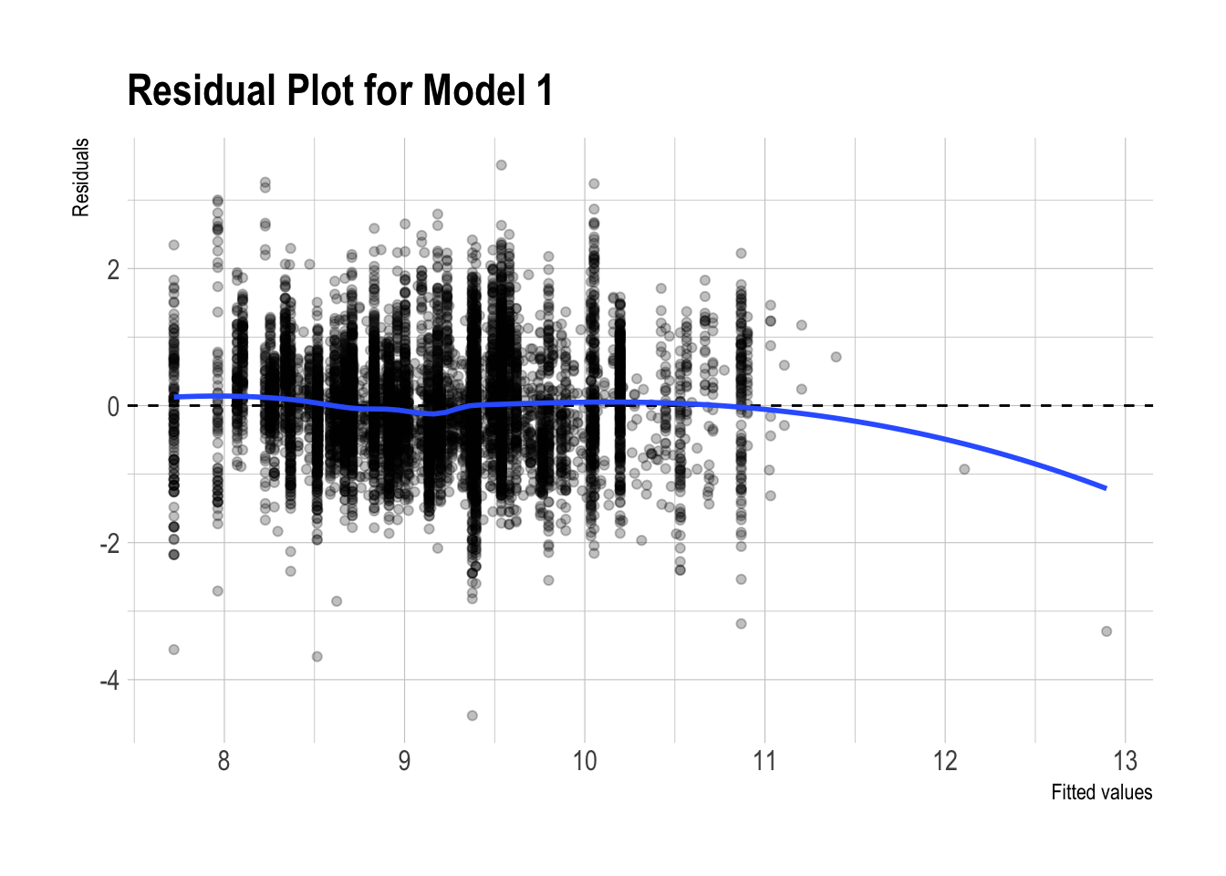
m3_r2 <- glance(m3)Residual Plots
m1_pred_test |>
  ggplot(aes(x = .fitted, y = .resid)) +
  geom_point(alpha = 0.25) +
  geom_hline(yintercept = 0, linetype = "dashed") +
  geom_smooth(se = FALSE, method = "loess") +
  labs(
    x = "Fitted values",
    y = "Residuals",
    title = "Residual Plot for Model 1"
  )
m2_pred_test |>
  ggplot(aes(x = .fitted, y = .resid)) +
  geom_point(alpha = 0.25) +
  geom_hline(yintercept = 0, linetype = "dashed") +
  geom_smooth(se = FALSE, method = "loess") +
  labs(
    x = "Fitted values",
    y = "Residuals",
    title = "Residual Plot for Model 2"
  )
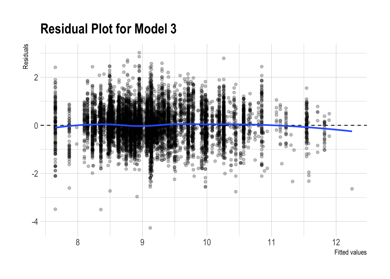
m3_pred_test |>
  ggplot(aes(x = .fitted, y = .resid)) +
  geom_point(alpha = 0.25) +
  geom_hline(yintercept = 0, linetype = "dashed") +
  geom_smooth(se = FALSE, method = "loess") +
  labs(
    x = "Fitted values",
    y = "Residuals",
    title = "Residual Plot for Model 3"
  )
RMSEs
RMSEs <- dtest |>
  mutate(
    resid_1 = log(sales) - pred_1,
    resid_2 = log(sales) - pred_2,
    resid_3 = log(sales) - pred_3
  ) |>
  summarize(
    rmse_1 = sqrt( mean( resid_1^2 ) ),
    rmse_2 = sqrt( mean( resid_2^2 ) ),
    rmse_3 = sqrt( mean( resid_3^2 ) )
  )

RMSEs
# A tibble: 1 × 3
rmse_1 rmse_2 rmse_3
<dbl> <dbl> <dbl>
1 0.791 0.790 0.690