library(tidyverse)
library(broom)
library(stargazer)
library(skimr)
library(DT)Linear Regression I
Bikeshare Data
R packages
Reading a CSV File
bikeshare <- read_csv('https://bcdanl.github.io/data/bikeshare_cleaned.csv')Variable description
| Variable | Description |
|---|---|
cnt |
Count of total rental bikes |
year |
Year |
month |
Month |
date |
Date |
hr |
Hour |
wkday |
Weekday |
holiday |
Holiday indicator (1 if holiday, 0 otherwise) |
seasons |
Season |
weather_cond |
Weather condition |
temp |
Temperature (measured in standard deviations from average) |
hum |
Humidity (measured in standard deviations from average) |
windspeed |
Wind speed (measured in standard deviations from average) |
Continuous variables
cnttemphumwindspeed
Categorical variables
yearmonthdatehrwkdayholidayseasonsweather_cond
Descriptive Statistics
skim(bikeshare)| Name | bikeshare |
| Number of rows | 17376 |
| Number of columns | 12 |
| _______________________ | |
| Column type frequency: | |
| character | 5 |
| numeric | 7 |
| ________________________ | |
| Group variables | None |
Variable type: character
| skim_variable | n_missing | complete_rate | min | max | empty | n_unique | whitespace |
|---|---|---|---|---|---|---|---|
| month | 0 | 1 | 2 | 2 | 0 | 12 | 0 |
| date | 0 | 1 | 2 | 2 | 0 | 31 | 0 |
| wkday | 0 | 1 | 6 | 9 | 0 | 7 | 0 |
| seasons | 0 | 1 | 4 | 6 | 0 | 4 | 0 |
| weather_cond | 0 | 1 | 14 | 24 | 0 | 3 | 0 |
Variable type: numeric
| skim_variable | n_missing | complete_rate | mean | sd | p0 | p25 | p50 | p75 | p100 | hist |
|---|---|---|---|---|---|---|---|---|---|---|
| cnt | 0 | 1 | 189.48 | 181.40 | 1.00 | 40.00 | 142.00 | 281.00 | 977.00 | ▇▃▁▁▁ |
| year | 0 | 1 | 2011.50 | 0.50 | 2011.00 | 2011.00 | 2012.00 | 2012.00 | 2012.00 | ▇▁▁▁▇ |
| hr | 0 | 1 | 11.55 | 6.91 | 0.00 | 6.00 | 12.00 | 18.00 | 23.00 | ▇▇▆▇▇ |
| holiday | 0 | 1 | 0.03 | 0.17 | 0.00 | 0.00 | 0.00 | 0.00 | 1.00 | ▇▁▁▁▁ |
| temp | 0 | 1 | 0.00 | 1.00 | -2.48 | -0.82 | 0.02 | 0.85 | 2.61 | ▂▇▇▇▁ |
| hum | 0 | 1 | 0.00 | 1.00 | -3.25 | -0.76 | 0.01 | 0.79 | 1.93 | ▁▃▇▇▆ |
| windspeed | 0 | 1 | 0.00 | 1.00 | -1.55 | -0.70 | 0.03 | 0.52 | 5.40 | ▇▆▂▁▁ |
Histograms
bikeshare |>
ggplot(aes(x = cnt)) +
geom_histogram()
Categorical Variables
bikeshare |>
count(year) |>
datatable()bikeshare |>
count(month) |>
datatable()bikeshare |>
count(date) |>
datatable()bikeshare |>
count(hr) |>
datatable()bikeshare |>
count(wkday) |>
datatable()bikeshare |>
count(holiday) |>
datatable()bikeshare |>
count(seasons) |>
datatable()bikeshare |>
count(weather_cond) |>
datatable()Data Preparation
bikeshare <- bikeshare |>
mutate(year = factor(year),
year = fct_relevel(year, "2011"),
seasons = factor(seasons,
levels =
c("spring",
"summer",
"fall",
"winter")),
month = factor(month),
month = fct_relevel(month, "01"),
hr = factor(hr,
levels = 0:23),
wkday = factor(wkday,
levels =
c("sunday", "monday", "tuesday", "wednesday",
"thursday", "friday", "saturday")),
weather_cond = factor(weather_cond,
levels =
c("Clear or Few Cloudy",
"Light Snow or Light Rain",
"Mist or Cloudy")),
)Training and Test Data
set.seed(1)
bikeshare <- bikeshare |>
mutate(rnd = runif(n()))
dtrain <- bikeshare |>
filter(rnd > 0.4)
dtest <- bikeshare |>
filter(rnd <= 0.4)
nrow(dtrain) / nrow(bikeshare)[1] 0.5965124Linear Regression Model
\[ \begin{align} \text{cnt}_{i} =\ &\beta_{\text{intercept}}\\ &+ \beta_{\text{temp}} \, \text{temp}_{i} + \beta_{\text{hum}} \, \text{hum}_{i} + \beta_{\text{windspeed}} \, \text{windspeed}_{i} \nonumber \\ &+ \beta_{\text{year\_2012}} \, \text{year\_2012}_{i}\\ &+ \beta_{\text{month\_2}} \, \text{month\_2}_{i} + \beta_{\text{month\_3}} \, \text{month\_3}_{i} + \beta_{\text{month\_4}} \, \text{month\_4}_{i} \nonumber \\ &+ \beta_{\text{month\_5}} \, \text{month\_5}_{i} + \beta_{\text{month\_6}} \, \text{month\_6}_{i} + \beta_{\text{month\_7}} \, \text{month\_7}_{i} + \beta_{\text{month\_8}} \, \text{month\_8}_{i} \nonumber \\ &+ \beta_{\text{month\_9}} \, \text{month\_9}_{i} + \beta_{\text{month\_10}} \, \text{month\_10}_{i} + \beta_{\text{month\_11}} \, \text{month\_11}_{i} + \beta_{\text{month\_12}} \, \text{month\_12}_{i} \nonumber \\ &+ \beta_{\text{hr\_1}} \, \text{hr\_1}_{i} + \beta_{\text{hr\_2}} \, \text{hr\_2}_{i} + \beta_{\text{hr\_3}} \, \text{hr\_3}_{i} + \beta_{\text{hr\_4}} \, \text{hr\_4}_{i} \nonumber \\ &+ \beta_{\text{hr\_5}} \, \text{hr\_5}_{i} + \beta_{\text{hr\_6}} \, \text{hr\_6}_{i} + \beta_{\text{hr\_7}} \, \text{hr\_7}_{i} + \beta_{\text{hr\_8}} \, \text{hr\_8}_{i} \nonumber \\ &+ \beta_{\text{hr\_9}} \, \text{hr\_9}_{i} + \beta_{\text{hr\_10}} \, \text{hr\_10}_{i} + \beta_{\text{hr\_11}} \, \text{hr\_11}_{i} + \beta_{\text{hr\_12}} \, \text{hr\_12}_{i} \nonumber \\ &+ \beta_{\text{hr\_13}} \, \text{hr\_13}_{i} + \beta_{\text{hr\_14}} \, \text{hr\_14}_{i} + \beta_{\text{hr\_15}} \, \text{hr\_15}_{i} + \beta_{\text{hr\_16}} \, \text{hr\_16}_{i} \nonumber \\ &+ \beta_{\text{hr\_17}} \, \text{hr\_17}_{i} + \beta_{\text{hr\_18}} \, \text{hr\_18}_{i} + \beta_{\text{hr\_19}} \, \text{hr\_19}_{i} + \beta_{\text{hr\_20}} \, \text{hr\_20}_{i} \nonumber \\ &+ \beta_{\text{hr\_21}} \, \text{hr\_21}_{i} + \beta_{\text{hr\_22}} \, \text{hr\_22}_{i} + \beta_{\text{hr\_23}} \, \text{hr\_23}_{i} \nonumber \\ &+ \beta_{\text{wkday\_monday}} \, \text{wkday\_monday}_{i} + \beta_{\text{wkday\_tuesday}} \, \text{wkday\_tuesday}_{i} + \beta_{\text{wkday\_wednesday}} \, \text{wkday\_wednesday}_{i} \nonumber \\ &+ \beta_{\text{wkday\_thursday}} \, \text{wkday\_thursday}_{i} + \beta_{\text{wkday\_friday}} \, \text{wkday\_friday}_{i} + \beta_{\text{wkday\_saturday}} \, \text{wkday\_saturday}_{i} \nonumber \\ &+ \beta_{\text{holiday\_1}} \, \text{holiday\_1}_{i} \nonumber \\ &+ \beta_{\text{seasons\_summer}} \, \text{seasons\_summer}_{i} + \beta_{\text{seasons\_fall}} \, \text{seasons\_fall}_{i} + \beta_{\text{seasons\_winter}} \, \text{seasons\_winter}_{i} \nonumber \\ &+ \beta_{\text{weather\_cond\_Light\_Snow\_or\_Light\_Rain}} \, \text{weather\_cond\_Light\_Snow\_or\_Light\_Rain}_{i}\nonumber \\ &+ \beta_{\text{weather\_cond\_Mist\_or\_Cloudy}} \, \text{weather\_cond\_Mist\_or\_Cloudy}_{i}\\ &+ \epsilon_{i} \end{align} \]
Note that all predictors are dummy variables, except for temp, hum, and windspeed.
Training the Model
model <- lm(cnt ~ temp + hum + windspeed +
year +
month +
hr +
wkday +
holiday +
seasons +
weather_cond,
data = dtrain)Regression Table with stargazer()
stargazer(model, type = "html")| Dependent variable: | |
| cnt | |
| temp | 45.480*** |
| (2.350) | |
| hum | -17.192*** |
| (1.386) | |
| windspeed | -4.965*** |
| (1.083) | |
| year2012 | 86.236*** |
| (2.026) | |
| month02 | 4.601 |
| (5.103) | |
| month03 | 10.228* |
| (5.705) | |
| month04 | 3.197 |
| (8.457) | |
| month05 | 17.549* |
| (9.049) | |
| month06 | 3.907 |
| (9.302) | |
| month07 | -12.534 |
| (10.479) | |
| month08 | 8.047 |
| (10.143) | |
| month09 | 31.316*** |
| (9.047) | |
| month10 | 13.305 |
| (8.429) | |
| month11 | -13.280 |
| (8.110) | |
| month12 | -11.074* |
| (6.421) | |
| hr1 | -15.375** |
| (6.960) | |
| hr2 | -24.699*** |
| (6.939) | |
| hr3 | -40.640*** |
| (7.015) | |
| hr4 | -41.506*** |
| (7.036) | |
| hr5 | -24.365*** |
| (6.952) | |
| hr6 | 34.893*** |
| (6.883) | |
| hr7 | 166.134*** |
| (6.915) | |
| hr8 | 319.314*** |
| (6.965) | |
| hr9 | 162.039*** |
| (6.868) | |
| hr10 | 111.098*** |
| (6.932) | |
| hr11 | 137.942*** |
| (6.941) | |
| hr12 | 168.066*** |
| (7.012) | |
| hr13 | 164.771*** |
| (7.317) | |
| hr14 | 145.958*** |
| (7.153) | |
| hr15 | 165.300*** |
| (7.188) | |
| hr16 | 222.334*** |
| (7.217) | |
| hr17 | 378.852*** |
| (7.058) | |
| hr18 | 345.427*** |
| (7.064) | |
| hr19 | 233.315*** |
| (6.954) | |
| hr20 | 155.840*** |
| (7.014) | |
| hr21 | 108.184*** |
| (6.980) | |
| hr22 | 70.452*** |
| (6.943) | |
| hr23 | 27.440*** |
| (6.927) | |
| wkdaymonday | 8.383** |
| (3.865) | |
| wkdaytuesday | 11.273*** |
| (3.734) | |
| wkdaywednesday | 16.442*** |
| (3.732) | |
| wkdaythursday | 12.750*** |
| (3.757) | |
| wkdayfriday | 18.119*** |
| (3.719) | |
| wkdaysaturday | 16.427*** |
| (3.693) | |
| holiday | -31.995*** |
| (6.466) | |
| seasonssummer | 38.039*** |
| (6.275) | |
| seasonsfall | 25.825*** |
| (7.428) | |
| seasonswinter | 73.019*** |
| (6.360) | |
| weather_condLight Snow or Light Rain | -64.598*** |
| (4.145) | |
| weather_condMist or Cloudy | -10.930*** |
| (2.487) | |
| Constant | -19.330*** |
| (7.497) | |
| Observations | 10,365 |
| R2 | 0.692 |
| Adjusted R2 | 0.691 |
| Residual Std. Error | 101.607 (df = 10314) |
| F Statistic | 463.994*** (df = 50; 10314) |
| Note: | p<0.1; p<0.05; p<0.01 |
Beta Estimates with tidy()
model_betas <- tidy(model,
conf.int = T) # conf.level = 0.95 (default)
model_betas_90ci <- tidy(model,
conf.int = T,
conf.level = 0.90)
model_betas_99ci <- tidy(model,
conf.int = T,
conf.level = 0.99)
rmarkdown::paged_table(model_betas)# coef(model) returns a vector of beta estimates:
# coef(model)Prediction with augment()
model_pred_train <- augment(model)
rmarkdown::paged_table(model_pred_train)model_pred_test <- augment(model, newdata = dtest)
rmarkdown::paged_table(model_pred_test)Various Model Statistics with glance()
model_r2 <- glance(model)
rmarkdown::paged_table(model_r2)Coefficient Plots
model_betas |>
filter(str_detect(term, "hr")) |>
mutate(term = factor(term,
levels = str_c("hr", 1:23))
)|>
ggplot(
aes(xmin = conf.low,
xmax = conf.high,
x = estimate,
y = term)
) +
geom_pointrange() +
geom_point() +
geom_vline(xintercept = 0, color = "darkorange", linetype = 2) +
labs(y = "")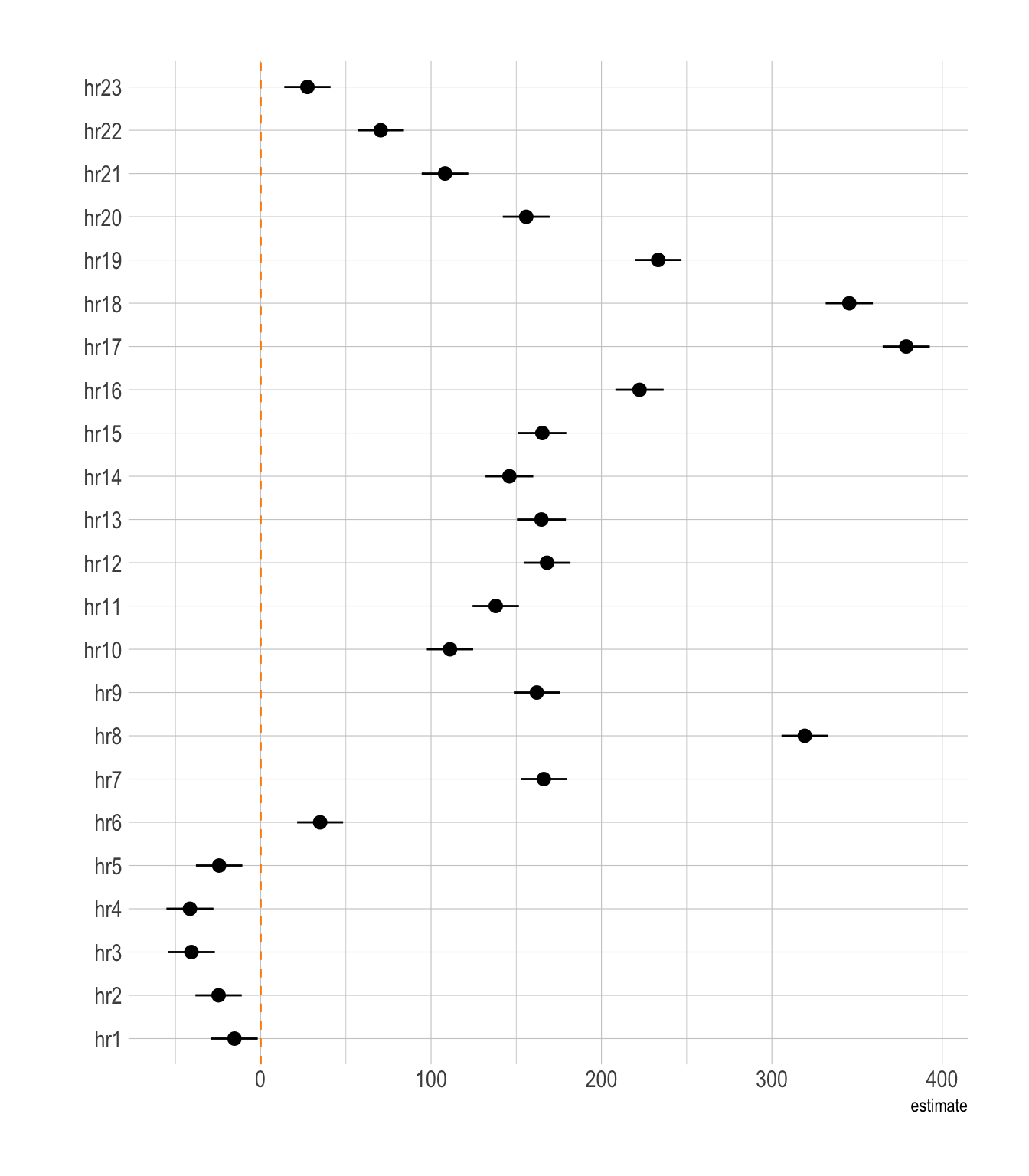
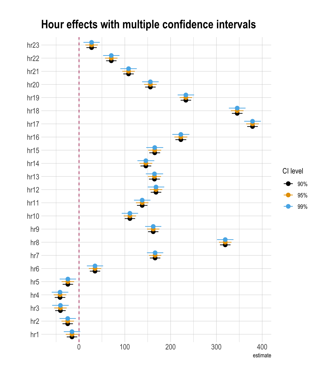
# Add a CI label to each and row-bind
month_ci <- bind_rows(
model_betas_90ci |> mutate(ci = "90%"),
model_betas |> mutate(ci = "95%"),
model_betas_99ci |> mutate(ci = "99%")
) |>
filter(str_detect(term, "hr")) |>
mutate(term = factor(term,
levels = str_c("hr", 1:23))
)|>
mutate(ci = factor(ci, levels = c("90%", "95%", "99%")))
ggplot(
month_ci,
aes(
y = term,
x = estimate,
xmin = conf.low,
xmax = conf.high,
color = ci
)
) +
geom_vline(xintercept = 0, color = "maroon", linetype = 2) +
geom_pointrange(
position = position_dodge(width = 0.6)
) +
labs(
title = "Hour effects with multiple confidence intervals",
color = "CI level",
y = ""
) 
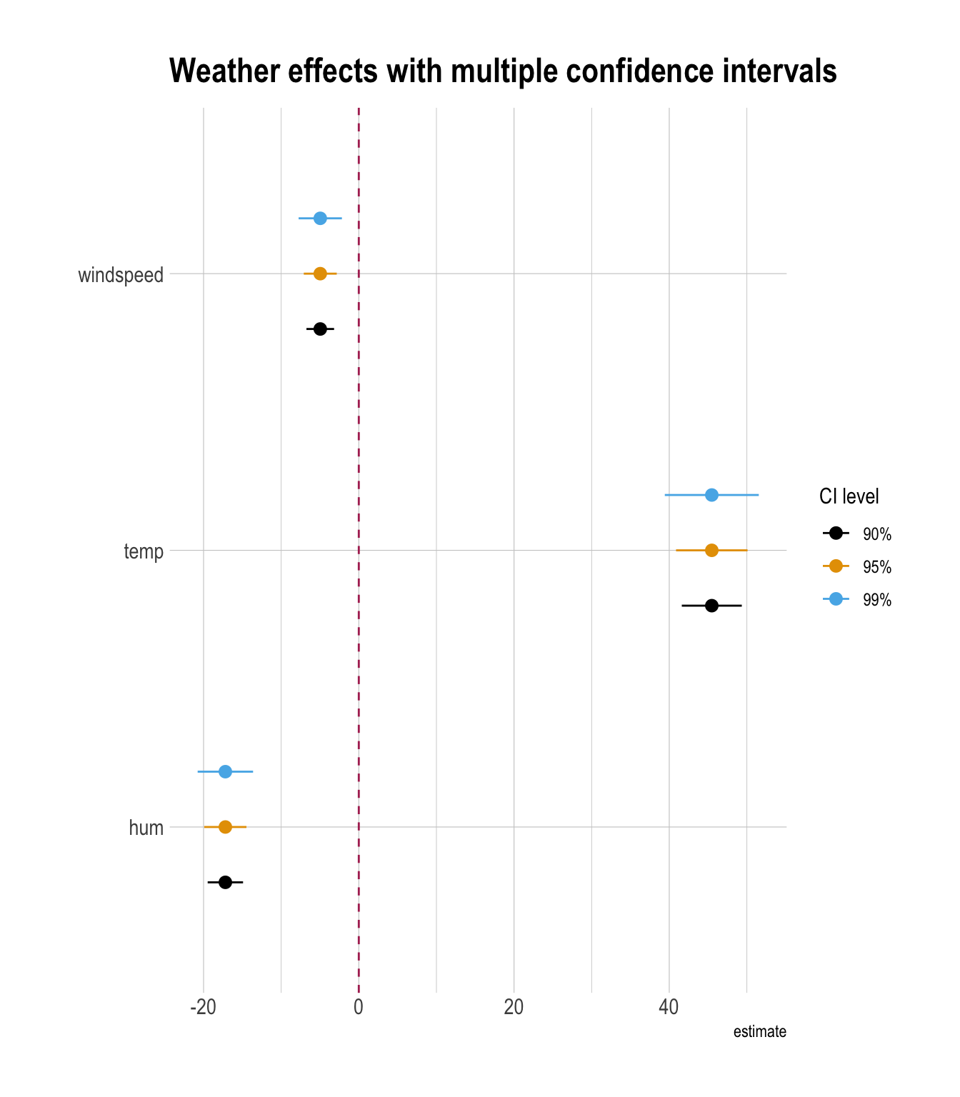
month_ci <- bind_rows(
model_betas_90ci |> mutate(ci = "90%"),
model_betas |> mutate(ci = "95%"),
model_betas_99ci |> mutate(ci = "99%")
) |>
filter(term %in% c("temp", "hum", "windspeed")) |>
mutate(ci = factor(ci, levels = c("90%", "95%", "99%")))
ggplot(
month_ci,
aes(
y = term,
x = estimate,
xmin = conf.low,
xmax = conf.high,
color = ci
)
) +
geom_vline(xintercept = 0, color = "maroon", linetype = 2) +
geom_pointrange(
position = position_dodge(width = 0.6)
) +
labs(
title = "Weather effects with multiple confidence intervals",
color = "CI level",
y = ""
) 
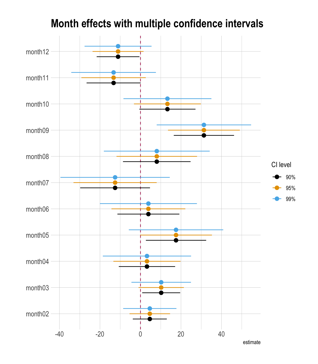
month_ci <- bind_rows(
model_betas_90ci |> mutate(ci = "90%"),
model_betas |> mutate(ci = "95%"),
model_betas_99ci |> mutate(ci = "99%")
) |>
filter(str_detect(term, "month")) |>
mutate(ci = factor(ci, levels = c("90%", "95%", "99%")))
ggplot(
month_ci,
aes(
y = term,
x = estimate,
xmin = conf.low,
xmax = conf.high,
color = ci
)
) +
geom_vline(xintercept = 0, color = "maroon", linetype = 2) +
geom_pointrange(
position = position_dodge(width = 0.6)
) +
labs(
title = "Month effects with multiple confidence intervals",
color = "CI level",
y = ""
) 
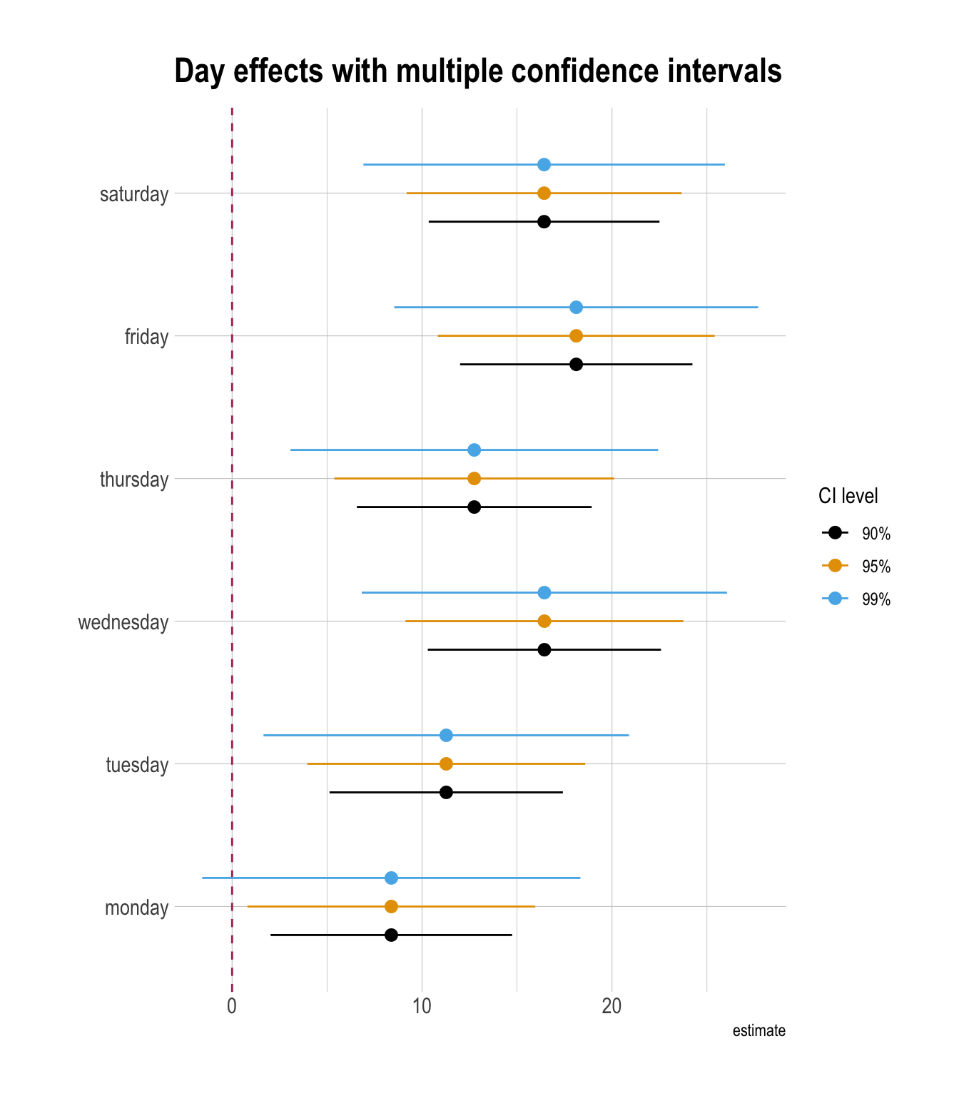
month_ci <- bind_rows(
model_betas_90ci |> mutate(ci = "90%"),
model_betas |> mutate(ci = "95%"),
model_betas_99ci |> mutate(ci = "99%")
) |>
filter(str_detect(term, "wkday")) |>
mutate(term = str_replace_all(term, "wkday", ""),
term = factor(term,
levels =
c("monday", "tuesday", "wednesday",
"thursday", "friday", "saturday"))) |>
mutate(ci = factor(ci, levels = c("90%", "95%", "99%")))
ggplot(
month_ci,
aes(
y = term,
x = estimate,
xmin = conf.low,
xmax = conf.high,
color = ci
)
) +
geom_vline(xintercept = 0, color = "maroon", linetype = 2) +
geom_pointrange(
position = position_dodge(width = 0.6)
) +
labs(
title = "Day effects with multiple confidence intervals",
color = "CI level",
y = ""
) 
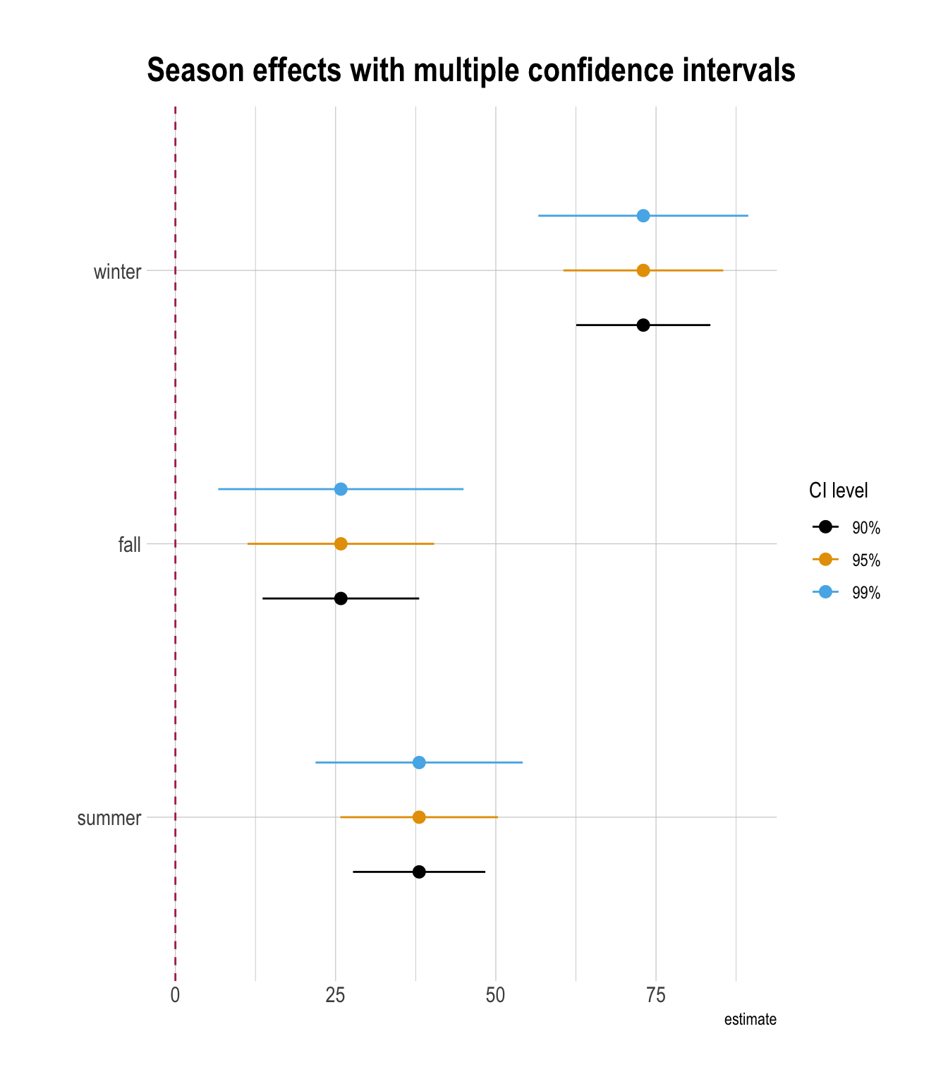
month_ci <- bind_rows(
model_betas_90ci |> mutate(ci = "90%"),
model_betas |> mutate(ci = "95%"),
model_betas_99ci |> mutate(ci = "99%")
) |>
filter(str_detect(term, "seasons")) |>
mutate(term = str_replace_all(term, "seasons", ""),
term = factor(term,
levels =
c("summer", "fall", "winter"))) |>
mutate(ci = factor(ci, levels = c("90%", "95%", "99%")))
ggplot(
month_ci,
aes(
y = term,
x = estimate,
xmin = conf.low,
xmax = conf.high,
color = ci
)
) +
geom_vline(xintercept = 0, color = "maroon", linetype = 2) +
geom_pointrange(
position = position_dodge(width = 0.6)
) +
labs(
title = "Season effects with multiple confidence intervals",
color = "CI level",
y = ""
) 
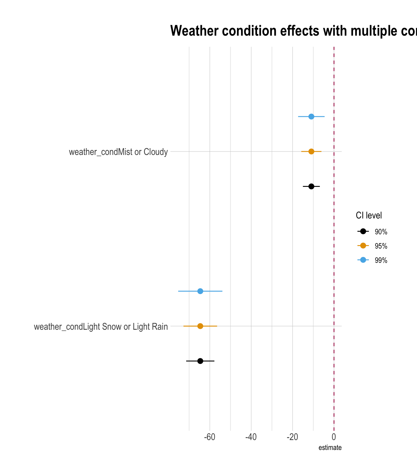
month_ci <- bind_rows(
model_betas_90ci |> mutate(ci = "90%"),
model_betas |> mutate(ci = "95%"),
model_betas_99ci |> mutate(ci = "99%")
) |>
filter(str_detect(term, "weather_cond")) |>
mutate(ci = factor(ci, levels = c("90%", "95%", "99%")))
ggplot(
month_ci,
aes(
y = term,
x = estimate,
xmin = conf.low,
xmax = conf.high,
color = ci
)
) +
geom_vline(xintercept = 0, color = "maroon", linetype = 2) +
geom_pointrange(
position = position_dodge(width = 0.6)
) +
labs(
title = "Weather condition effects with multiple confidence intervals",
color = "CI level",
y = ""
) 
Residual Plot
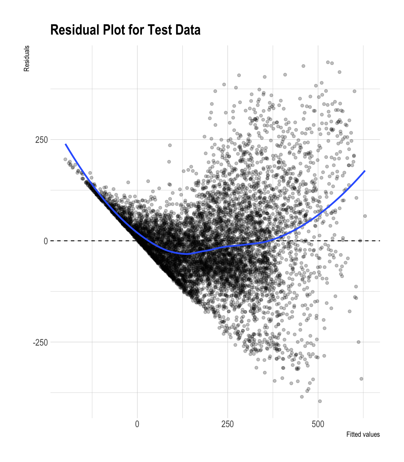
model_pred_test |>
ggplot(aes(x = .fitted, y = .resid)) +
geom_point(alpha = 0.25) +
geom_hline(yintercept = 0, linetype = "dashed") +
geom_smooth(se = FALSE, method = "loess") +
labs(
x = "Fitted values",
y = "Residuals",
title = "Residual Plot for Test Data"
)
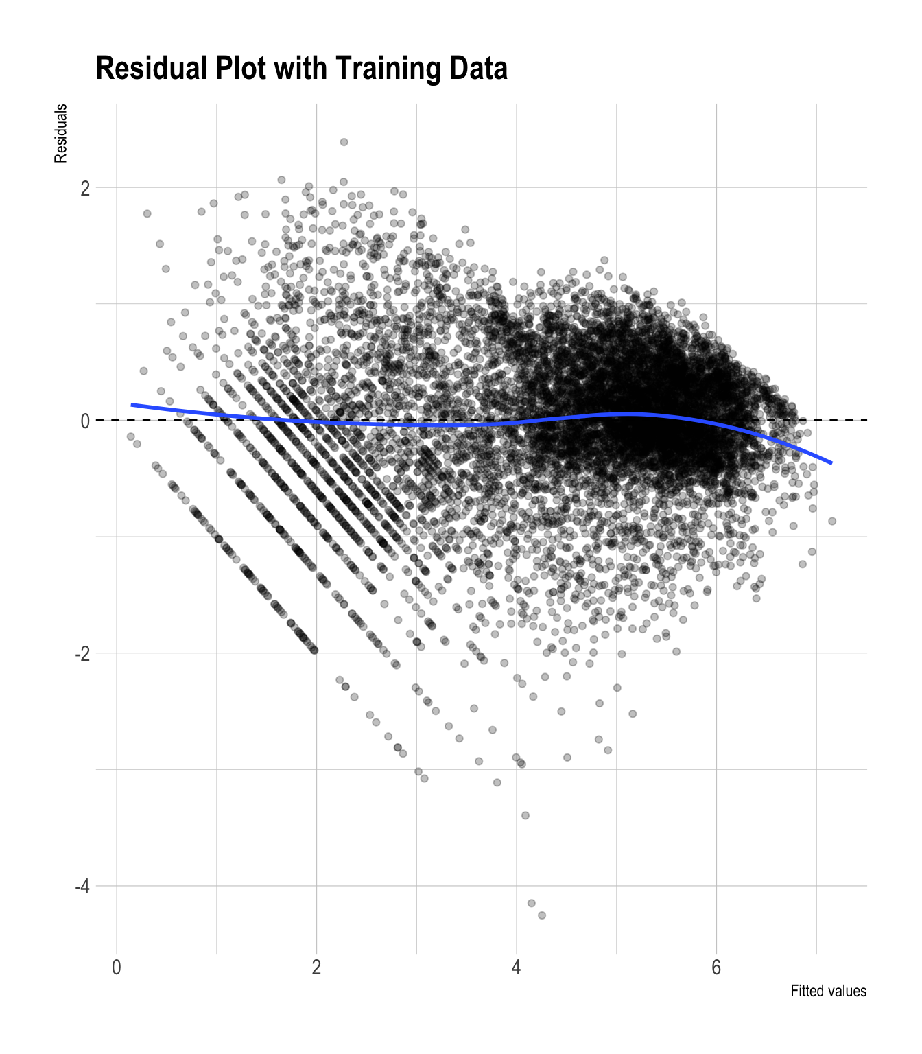
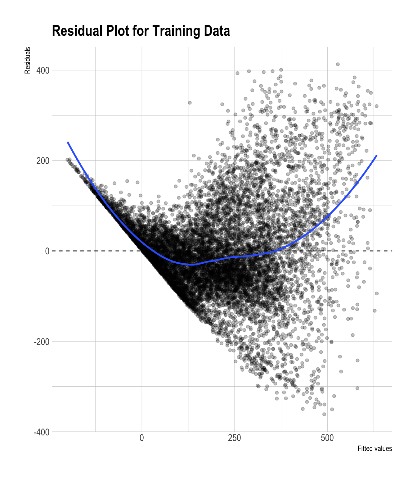
model_pred_train |>
ggplot(aes(x = .fitted, y = .resid)) +
geom_point(alpha = 0.25) +
geom_hline(yintercept = 0, linetype = "dashed") +
geom_smooth(se = FALSE, method = "loess") +
labs(
x = "Fitted values",
y = "Residuals",
title = "Residual Plot for Training Data"
)
Linear Regression Model with Log-Transformed Outcome
Histograms
bikeshare |>
ggplot(aes(x = cnt)) +
geom_histogram()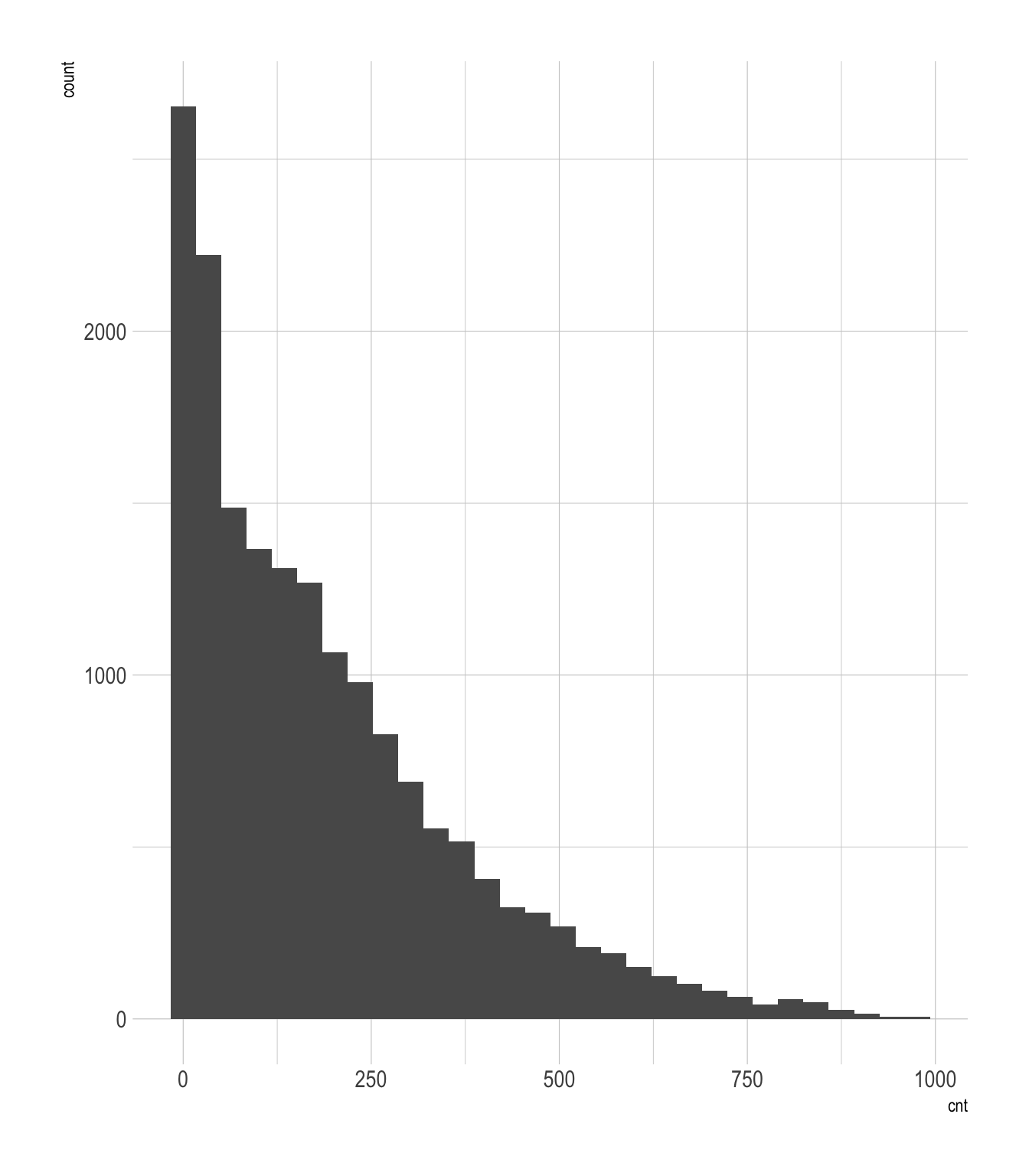
bikeshare |>
ggplot(aes(x = log(cnt))) +
geom_histogram()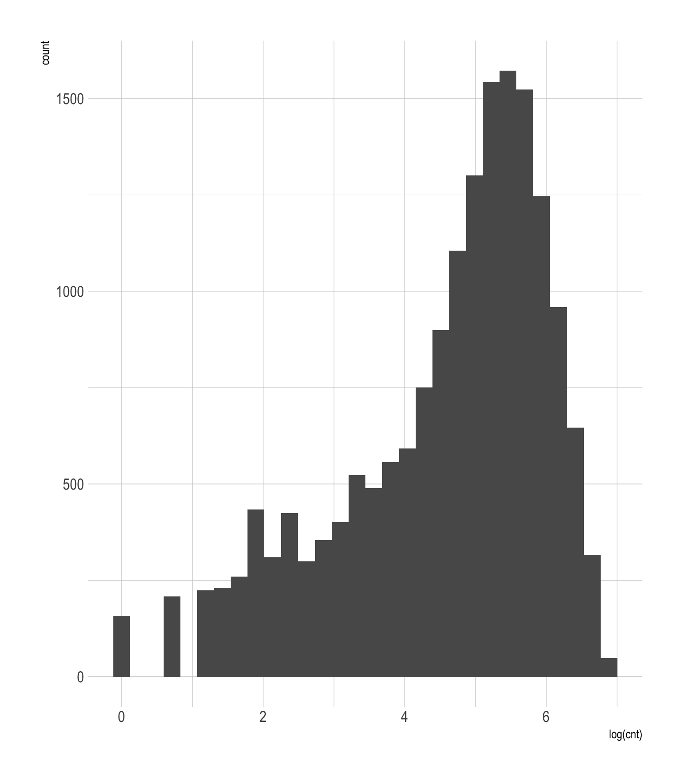
\[ \begin{align} \log(\text{cnt}_{i}) =\ &\beta_{\text{intercept}}\\ &+ \beta_{\text{temp}} \, \text{temp}_{i} + \beta_{\text{hum}} \, \text{hum}_{i} + \beta_{\text{windspeed}} \, \text{windspeed}_{i} \nonumber \\ &+ \beta_{\text{year\_2012}} \, \text{year\_2012}_{i}\\ &+ \beta_{\text{month\_2}} \, \text{month\_2}_{i} + \beta_{\text{month\_3}} \, \text{month\_3}_{i} + \beta_{\text{month\_4}} \, \text{month\_4}_{i} \nonumber \\ &+ \beta_{\text{month\_5}} \, \text{month\_5}_{i} + \beta_{\text{month\_6}} \, \text{month\_6}_{i} + \beta_{\text{month\_7}} \, \text{month\_7}_{i} + \beta_{\text{month\_8}} \, \text{month\_8}_{i} \nonumber \\ &+ \beta_{\text{month\_9}} \, \text{month\_9}_{i} + \beta_{\text{month\_10}} \, \text{month\_10}_{i} + \beta_{\text{month\_11}} \, \text{month\_11}_{i} + \beta_{\text{month\_12}} \, \text{month\_12}_{i} \nonumber \\ &+ \beta_{\text{hr\_1}} \, \text{hr\_1}_{i} + \beta_{\text{hr\_2}} \, \text{hr\_2}_{i} + \beta_{\text{hr\_3}} \, \text{hr\_3}_{i} + \beta_{\text{hr\_4}} \, \text{hr\_4}_{i} \nonumber \\ &+ \beta_{\text{hr\_5}} \, \text{hr\_5}_{i} + \beta_{\text{hr\_6}} \, \text{hr\_6}_{i} + \beta_{\text{hr\_7}} \, \text{hr\_7}_{i} + \beta_{\text{hr\_8}} \, \text{hr\_8}_{i} \nonumber \\ &+ \beta_{\text{hr\_9}} \, \text{hr\_9}_{i} + \beta_{\text{hr\_10}} \, \text{hr\_10}_{i} + \beta_{\text{hr\_11}} \, \text{hr\_11}_{i} + \beta_{\text{hr\_12}} \, \text{hr\_12}_{i} \nonumber \\ &+ \beta_{\text{hr\_13}} \, \text{hr\_13}_{i} + \beta_{\text{hr\_14}} \, \text{hr\_14}_{i} + \beta_{\text{hr\_15}} \, \text{hr\_15}_{i} + \beta_{\text{hr\_16}} \, \text{hr\_16}_{i} \nonumber \\ &+ \beta_{\text{hr\_17}} \, \text{hr\_17}_{i} + \beta_{\text{hr\_18}} \, \text{hr\_18}_{i} + \beta_{\text{hr\_19}} \, \text{hr\_19}_{i} + \beta_{\text{hr\_20}} \, \text{hr\_20}_{i} \nonumber \\ &+ \beta_{\text{hr\_21}} \, \text{hr\_21}_{i} + \beta_{\text{hr\_22}} \, \text{hr\_22}_{i} + \beta_{\text{hr\_23}} \, \text{hr\_23}_{i} \nonumber \\ &+ \beta_{\text{wkday\_monday}} \, \text{wkday\_monday}_{i} + \beta_{\text{wkday\_tuesday}} \, \text{wkday\_tuesday}_{i} + \beta_{\text{wkday\_wednesday}} \, \text{wkday\_wednesday}_{i} \nonumber \\ &+ \beta_{\text{wkday\_thursday}} \, \text{wkday\_thursday}_{i} + \beta_{\text{wkday\_friday}} \, \text{wkday\_friday}_{i} + \beta_{\text{wkday\_saturday}} \, \text{wkday\_saturday}_{i} \nonumber \\ &+ \beta_{\text{holiday\_1}} \, \text{holiday\_1}_{i} \nonumber \\ &+ \beta_{\text{seasons\_summer}} \, \text{seasons\_summer}_{i} + \beta_{\text{seasons\_fall}} \, \text{seasons\_fall}_{i} + \beta_{\text{seasons\_winter}} \, \text{seasons\_winter}_{i} \nonumber \\ &+ \beta_{\text{weather\_cond\_Light\_Snow\_or\_Light\_Rain}} \, \text{weather\_cond\_Light\_Snow\_or\_Light\_Rain}_{i}\nonumber \\ &+ \beta_{\text{weather\_cond\_Mist\_or\_Cloudy}} \, \text{weather\_cond\_Mist\_or\_Cloudy}_{i}\\ &+ \epsilon_{i} \end{align} \]
Training the Model
model_log <- lm(log(cnt) ~ temp + hum + windspeed +
year +
month +
hr +
wkday +
holiday +
seasons +
weather_cond,
data = dtrain)Regression Table with stargazer()
stargazer(model_log, type = "html")| Dependent variable: | |
| log(cnt) | |
| temp | 0.277*** |
| (0.014) | |
| hum | -0.057*** |
| (0.009) | |
| windspeed | -0.037*** |
| (0.007) | |
| year2012 | 0.486*** |
| (0.012) | |
| month02 | 0.146*** |
| (0.031) | |
| month03 | 0.114*** |
| (0.035) | |
| month04 | 0.064 |
| (0.052) | |
| month05 | 0.208*** |
| (0.056) | |
| month06 | 0.078 |
| (0.057) | |
| month07 | -0.093 |
| (0.065) | |
| month08 | 0.001 |
| (0.062) | |
| month09 | 0.070 |
| (0.056) | |
| month10 | -0.018 |
| (0.052) | |
| month11 | -0.097* |
| (0.050) | |
| month12 | -0.084** |
| (0.040) | |
| hr1 | -0.606*** |
| (0.043) | |
| hr2 | -1.125*** |
| (0.043) | |
| hr3 | -1.794*** |
| (0.043) | |
| hr4 | -2.021*** |
| (0.043) | |
| hr5 | -0.993*** |
| (0.043) | |
| hr6 | 0.241*** |
| (0.042) | |
| hr7 | 1.239*** |
| (0.043) | |
| hr8 | 1.916*** |
| (0.043) | |
| hr9 | 1.574*** |
| (0.042) | |
| hr10 | 1.252*** |
| (0.043) | |
| hr11 | 1.386*** |
| (0.043) | |
| hr12 | 1.524*** |
| (0.043) | |
| hr13 | 1.507*** |
| (0.045) | |
| hr14 | 1.413*** |
| (0.044) | |
| hr15 | 1.507*** |
| (0.044) | |
| hr16 | 1.730*** |
| (0.044) | |
| hr17 | 2.142*** |
| (0.043) | |
| hr18 | 2.042*** |
| (0.043) | |
| hr19 | 1.760*** |
| (0.043) | |
| hr20 | 1.480*** |
| (0.043) | |
| hr21 | 1.245*** |
| (0.043) | |
| hr22 | 0.984*** |
| (0.043) | |
| hr23 | 0.581*** |
| (0.043) | |
| wkdaymonday | -0.037 |
| (0.024) | |
| wkdaytuesday | -0.039* |
| (0.023) | |
| wkdaywednesday | -0.010 |
| (0.023) | |
| wkdaythursday | 0.036 |
| (0.023) | |
| wkdayfriday | 0.122*** |
| (0.023) | |
| wkdaysaturday | 0.109*** |
| (0.023) | |
| holiday | -0.156*** |
| (0.040) | |
| seasonssummer | 0.339*** |
| (0.039) | |
| seasonsfall | 0.406*** |
| (0.046) | |
| seasonswinter | 0.673*** |
| (0.039) | |
| weather_condLight Snow or Light Rain | -0.603*** |
| (0.026) | |
| weather_condMist or Cloudy | -0.054*** |
| (0.015) | |
| Constant | 3.145*** |
| (0.046) | |
| Observations | 10,365 |
| R2 | 0.824 |
| Adjusted R2 | 0.823 |
| Residual Std. Error | 0.626 (df = 10314) |
| F Statistic | 967.908*** (df = 50; 10314) |
| Note: | p<0.1; p<0.05; p<0.01 |
Beta Estimates with tidy()
model_log_betas <- tidy(model_log,
conf.int = T) # conf.level = 0.95 (default)
model_log_betas_90ci <- tidy(model_log,
conf.int = T,
conf.level = 0.90)
model_log_betas_99ci <- tidy(model_log,
conf.int = T,
conf.level = 0.99)# coef(model_log) returns a vector of beta estimates:
# coef(model_log)Prediction with augment()
model_log_pred_train <- augment(model_log)
model_log_pred_test <- augment(model_log, newdata = dtest)Various Model Statistics with glance()
model_log_r2 <- glance(model_log)Coefficient Plots
model_log_betas |>
filter(str_detect(term, "hr")) |>
mutate(term = factor(term,
levels = str_c("hr", 1:23))
)|>
ggplot(
aes(xmin = exp(conf.low),
xmax = exp(conf.high),
x = exp(estimate),
y = term)
) +
geom_pointrange() +
geom_point() +
geom_vline(xintercept = 1, color = "darkorange", linetype = 2) +
labs(y = "")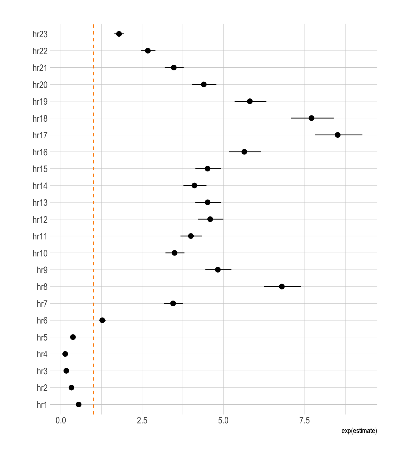
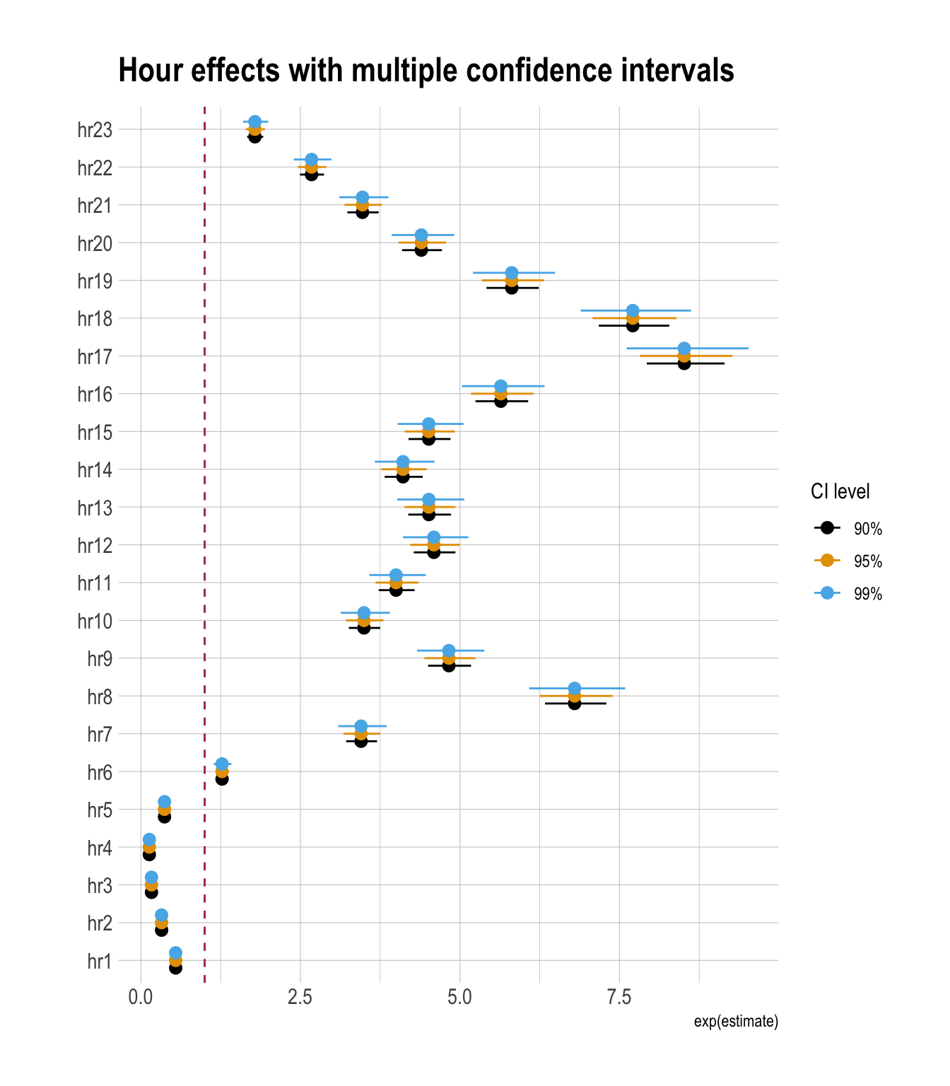
month_ci <- bind_rows(
model_log_betas_90ci |> mutate(ci = "90%"),
model_log_betas |> mutate(ci = "95%"),
model_log_betas_99ci |> mutate(ci = "99%")
) |>
filter(str_detect(term, "hr")) |>
mutate(term = factor(term,
levels = str_c("hr", 1:23))
)|>
mutate(ci = factor(ci, levels = c("90%", "95%", "99%")))
ggplot(
month_ci,
aes(
y = term,
x = exp(estimate),
xmin = exp(conf.low),
xmax = exp(conf.high),
color = ci
)
) +
geom_vline(xintercept = 1, color = "maroon", linetype = 2) +
geom_pointrange(
position = position_dodge(width = 0.6)
) +
labs(
title = "Hour effects with multiple confidence intervals",
color = "CI level",
y = ""
) 
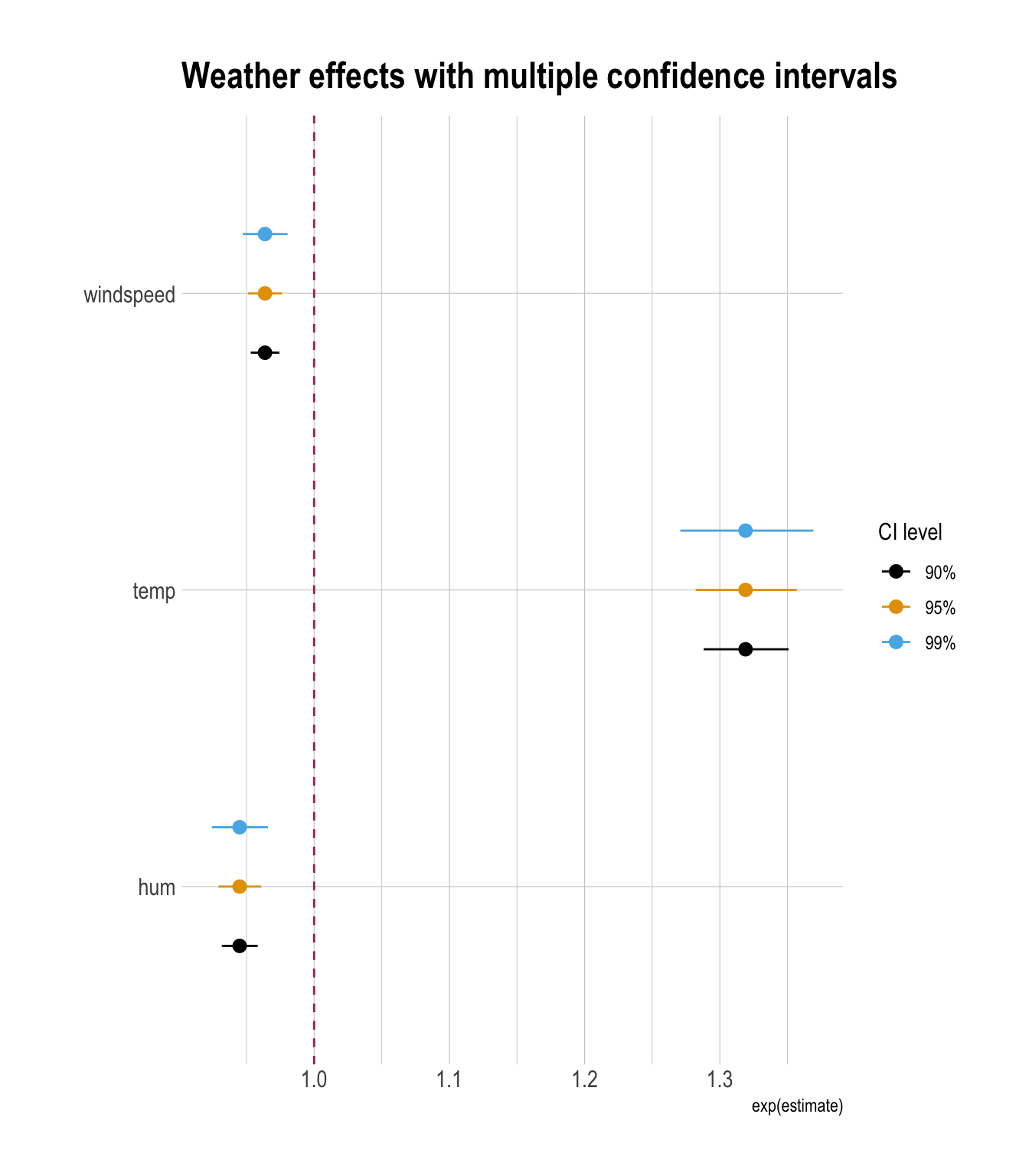
month_ci <- bind_rows(
model_log_betas_90ci |> mutate(ci = "90%"),
model_log_betas |> mutate(ci = "95%"),
model_log_betas_99ci |> mutate(ci = "99%")
) |>
filter(term %in% c("temp", "hum", "windspeed")) |>
mutate(ci = factor(ci, levels = c("90%", "95%", "99%")))
ggplot(
month_ci,
aes(
y = term,
x = exp(estimate),
xmin = exp(conf.low),
xmax = exp(conf.high),
color = ci
)
) +
geom_vline(xintercept = 1, color = "maroon", linetype = 2) +
geom_pointrange(
position = position_dodge(width = 0.6)
) +
labs(
title = "Weather effects with multiple confidence intervals",
color = "CI level",
y = ""
) 
month_ci <- bind_rows(
model_log_betas_90ci |> mutate(ci = "90%"),
model_log_betas |> mutate(ci = "95%"),
model_log_betas_99ci |> mutate(ci = "99%")
) |>
filter(str_detect(term, "month")) |>
mutate(ci = factor(ci, levels = c("90%", "95%", "99%")))
ggplot(
month_ci,
aes(
y = term,
x = exp(estimate),
xmin = exp(conf.low),
xmax = exp(conf.high),
color = ci
)
) +
geom_vline(xintercept = 1, color = "maroon", linetype = 2) +
geom_pointrange(
position = position_dodge(width = 0.6)
) +
labs(
title = "Month effects with multiple confidence intervals",
color = "CI level",
y = ""
) 
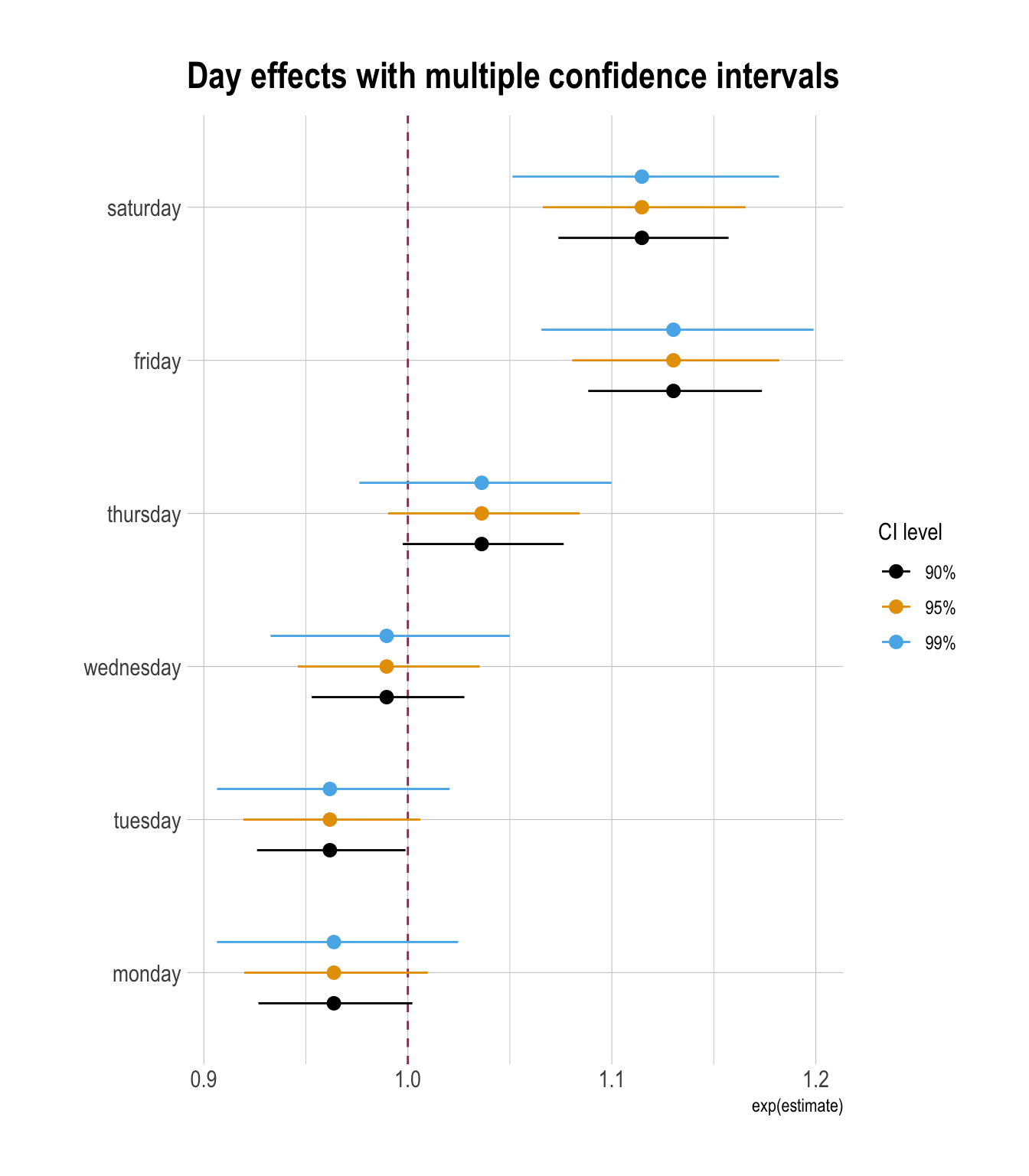
month_ci <- bind_rows(
model_log_betas_90ci |> mutate(ci = "90%"),
model_log_betas |> mutate(ci = "95%"),
model_log_betas_99ci |> mutate(ci = "99%")
) |>
filter(str_detect(term, "wkday")) |>
mutate(term = str_replace_all(term, "wkday", ""),
term = factor(term,
levels =
c("monday", "tuesday", "wednesday",
"thursday", "friday", "saturday"))) |>
mutate(ci = factor(ci, levels = c("90%", "95%", "99%")))
ggplot(
month_ci,
aes(
y = term,
x = exp(estimate),
xmin = exp(conf.low),
xmax = exp(conf.high),
color = ci
)
) +
geom_vline(xintercept = 1, color = "maroon", linetype = 2) +
geom_pointrange(
position = position_dodge(width = 0.6)
) +
labs(
title = "Day effects with multiple confidence intervals",
color = "CI level",
y = ""
) 
month_ci <- bind_rows(
model_log_betas_90ci |> mutate(ci = "90%"),
model_log_betas |> mutate(ci = "95%"),
model_log_betas_99ci |> mutate(ci = "99%")
) |>
filter(str_detect(term, "seasons")) |>
mutate(term = str_replace_all(term, "seasons", ""),
term = factor(term,
levels =
c("summer", "fall", "winter"))) |>
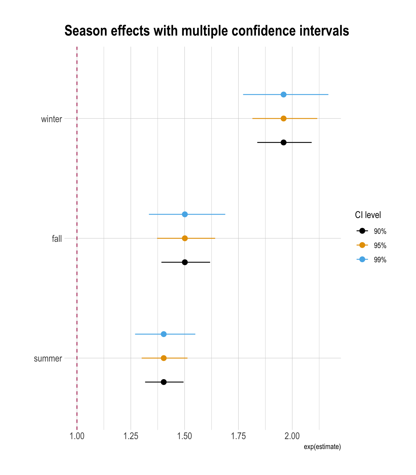
mutate(ci = factor(ci, levels = c("90%", "95%", "99%")))
ggplot(
month_ci,
aes(
y = term,
x = exp(estimate),
xmin = exp(conf.low),
xmax = exp(conf.high),
color = ci
)
) +
geom_vline(xintercept = 1, color = "maroon", linetype = 2) +
geom_pointrange(
position = position_dodge(width = 0.6)
) +
labs(
title = "Season effects with multiple confidence intervals",
color = "CI level",
y = ""
) 
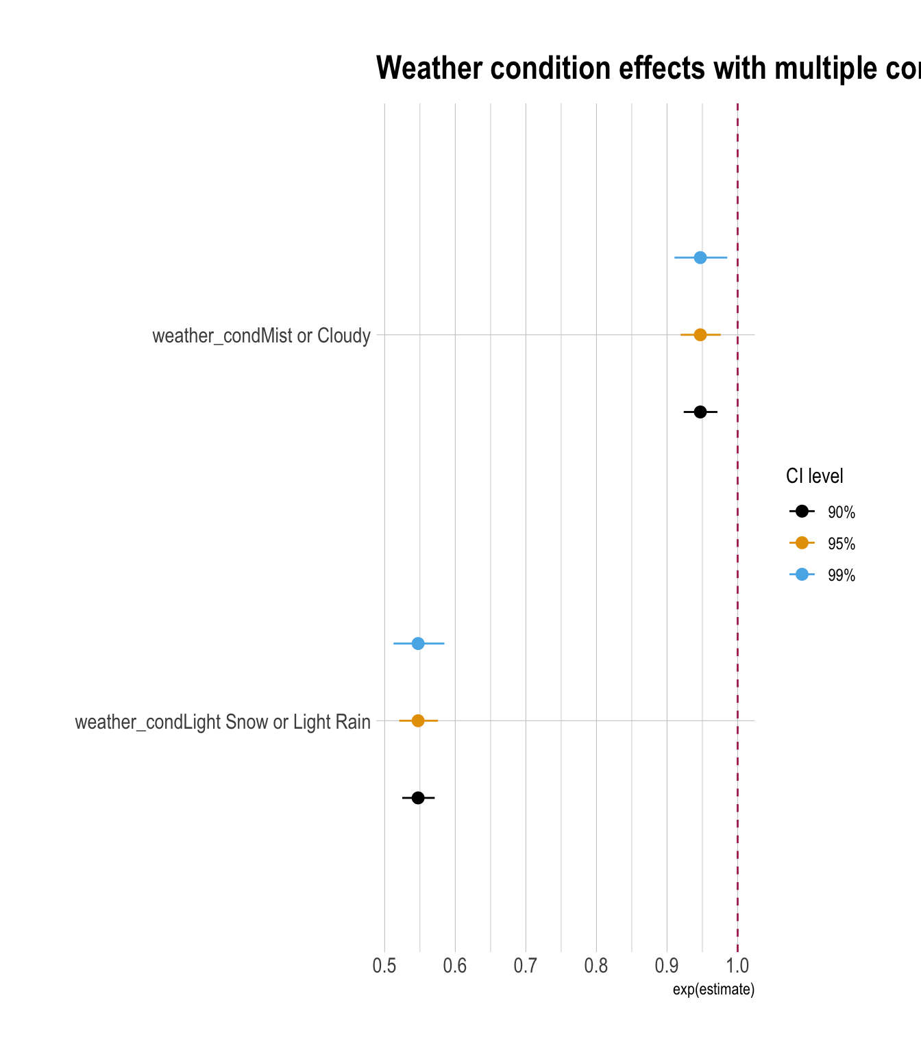
month_ci <- bind_rows(
model_log_betas_90ci |> mutate(ci = "90%"),
model_log_betas |> mutate(ci = "95%"),
model_log_betas_99ci |> mutate(ci = "99%")
) |>
filter(str_detect(term, "weather_cond")) |>
mutate(ci = factor(ci, levels = c("90%", "95%", "99%")))
ggplot(
month_ci,
aes(
y = term,
x = exp(estimate),
xmin = exp(conf.low),
xmax = exp(conf.high),
color = ci
)
) +
geom_vline(xintercept = 1, color = "maroon", linetype = 2) +
geom_pointrange(
position = position_dodge(width = 0.6)
) +
labs(
title = "Weather condition effects with multiple confidence intervals",
color = "CI level",
y = ""
) 
Residual Plot
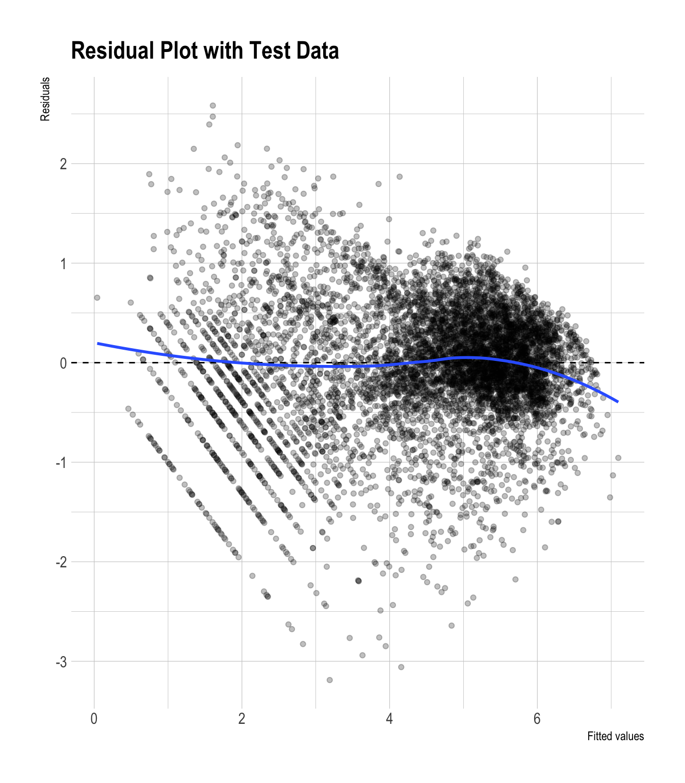
model_log_pred_test |>
ggplot(aes(x = .fitted, y = .resid)) +
geom_point(alpha = 0.25) +
geom_hline(yintercept = 0, linetype = "dashed") +
geom_smooth(se = FALSE, method = "loess") +
labs(
x = "Fitted values",
y = "Residuals",
title = "Residual Plot with Test Data"
)
model_log_pred_train |>
ggplot(aes(x = .fitted, y = .resid)) +
geom_point(alpha = 0.25) +
geom_hline(yintercept = 0, linetype = "dashed") +
geom_smooth(se = FALSE, method = "loess") +
labs(
x = "Fitted values",
y = "Residuals",
title = "Residual Plot with Training Data"
)