library(tidyverse)
library(janitor)
library(ggthemes)
library(rmarkdown)

library(rpart)
library(rpart.plot)
library(vip)
library(pdp)

theme_set(
  theme_bw() +
    theme(
      legend.position = "bottom",
      strip.background = element_rect(fill = "lightgray"),
      axis.title.x = element_text(size = rel(1.1)),
      axis.title.y = element_text(size = rel(1.1))
    )
)

scale_colour_discrete <- function(...) scale_color_colorblind(...)
scale_fill_discrete <- function(...) scale_fill_colorblind(...)Decision Trees
NBC Show Data
Setup for Decision Trees
NBC Show Data
nbc <- read_csv("https://bcdanl.github.io/data/nbc_show.csv") |>
  janitor::clean_names()  # column names are with all lowercase;
                          # spaces in column names are replaced by _

paged_table(nbc)- GRP: Gross Ratings Points, an estimate of total viewership or broadcast marketability
- PE: Projected Engagement, based on viewer recall of order and detail after watching the show
nbc_demog <- read_csv("https://bcdanl.github.io/data/nbc_demog.csv") |>
janitor::clean_names()
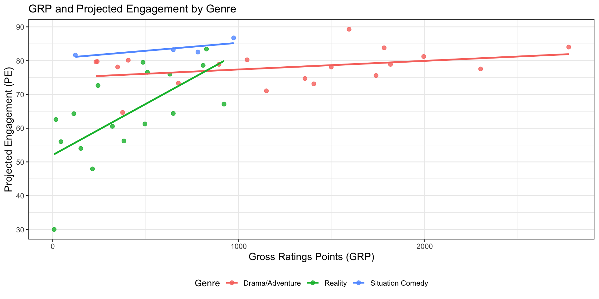
paged_table(nbc_demog)Visualize GRP and PE by genre
nbc |>
  ggplot(aes(x = grp, y = pe, color = genre)) +
  geom_point(size = 2, alpha = 0.8) +
  geom_smooth(method = "lm", se = FALSE) +
  labs(
    title = "GRP and Projected Engagement by Genre",
    x = "Gross Ratings Points (GRP)",
    y = "Projected Engagement (PE)",
    color = "Genre"
  )
Regression Tree
Modeling goal
- Predict
peusinggrpandgenre - This is a regression tree because
peis numeric - The tree will allow nonlinear relationships and interactions between audience size and show genre
Fit the initial regression tree using rpart()
init_nbc_tree <- rpart(
  pe ~ grp + genre,
  data = nbc,
  method = "anova"
)
Key arguments in rpart()
formula: specifies the outcome and predictorsdata: the data frame used for estimationmethod = "anova": use a regression tree for a numeric outcomemethod = "class": use a classification tree for a categorical outcomecontrol = rpart.control(...): determines how aggressively the tree is allowed to grow
How to interpret the rpart output for a regression tree
init_nbc_treen= 40
node), split, n, deviance, yval
* denotes terminal node
1) root 40 5646.4560 72.68308
2) grp< 223.05 7 1512.7210 56.63661 *
3) grp>=223.05 33 1948.9810 76.08687
6) genre=Reality 11 823.4392 70.56522 *
7) genre=Drama/Adventure,Situation Comedy 22 622.4796 78.84770
14) grp< 1545.15 15 421.4750 77.61867 *
15) grp>=1545.15 7 129.7948 81.48133 *node)= node number in the tree- The node numbers follow a binary tree indexing convention — the same system used in binary heaps. For any node numbered \(n\):
- Its left child is \(2n\)
- Its right child is \(2n + 1\)
- The node numbers follow a binary tree indexing convention — the same system used in binary heaps. For any node numbered \(n\):
split= the rule used to divide the data at that noden= number of observations in that nodedeviance= the sum of squared errors within that node for a regression treeyval= the predicted value at that node, which is the mean outcome for observations in the node*denotes a terminal node, also called a leaf node
How to read the plotted tree
rpart.plot(init_nbc_tree)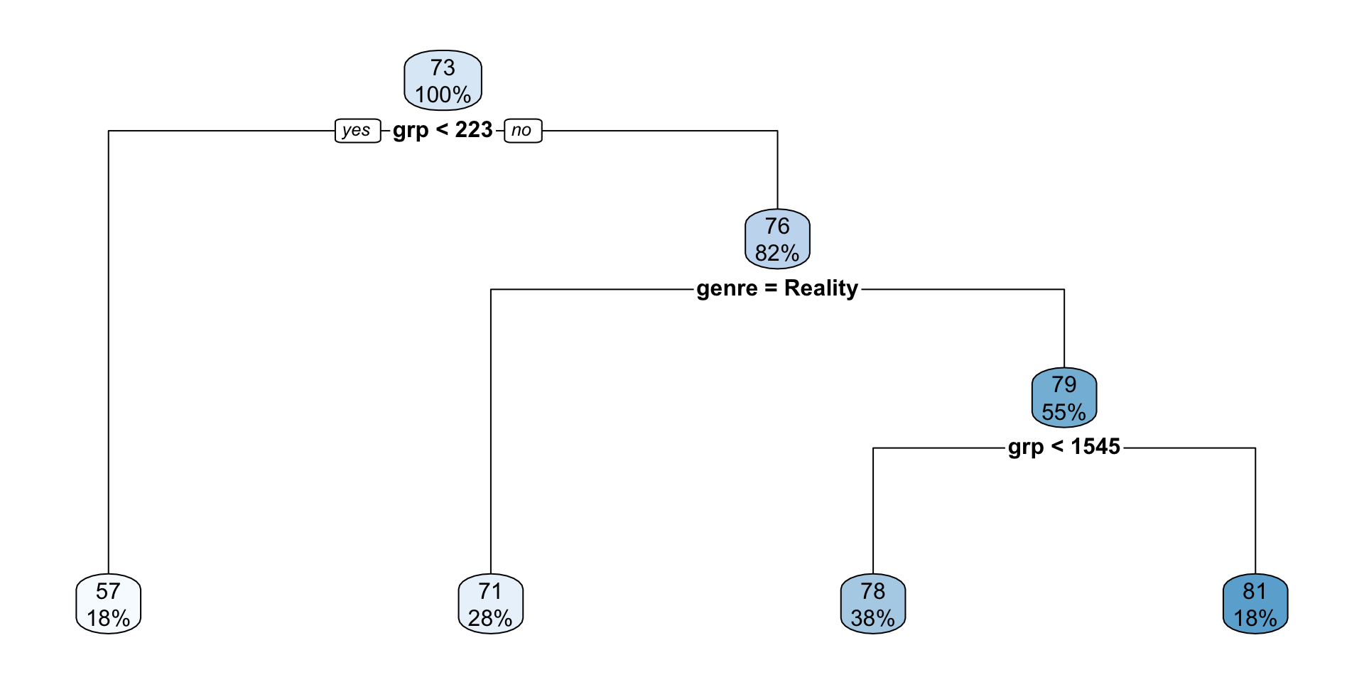
- Start at the root node at the top.
- Read the split rule.
- Observations satisfying the rule go left, and the rest go right.
- Continue until you reach a leaf.
- The two numbers in each node are:
- the predicted value (\(\widehat{y}\)) for that node
- the percentage of observations in that node
plotcp() for an rpart tree
plotcp(init_nbc_tree)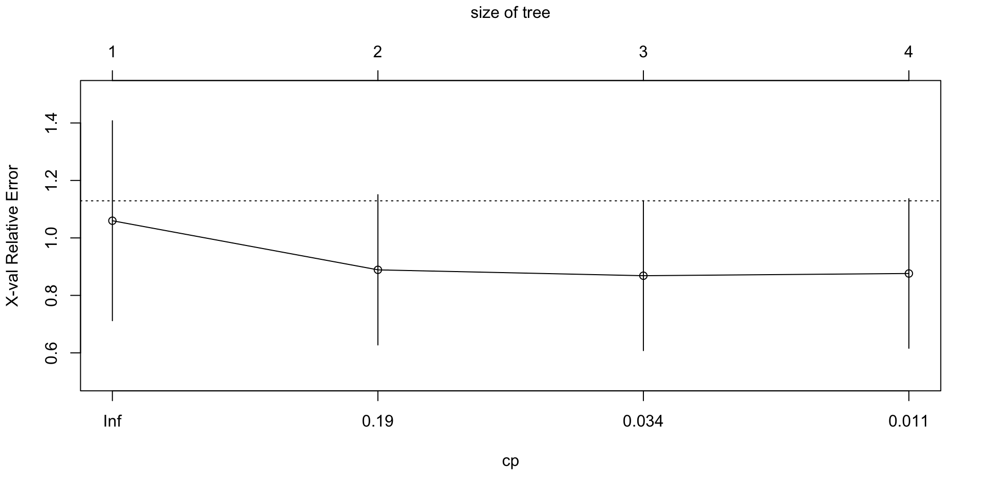
plotcp()visualizes the cost-complexity pruning results stored in the fittedrpartobject.The horizontal axis shows the size of the tree, often in terms of the number of splits.
The vertical axis shows the cross-validated error, labeled
xerror.Lower values of
xerrorindicate better estimated out-of-sample performance.Each point represents a candidate pruning level, indexed by the complexity parameter
cp.The vertical bars show uncertainty around the cross-validated error using
xstd, the estimated standard error.A very large tree may fit the training data well but still have higher cross-validated error.
A smaller pruned tree is often preferred if it achieves similar or lower cross-validated error.
The size of the tree refers to the number of splits, or internal decision nodes, in the tree.
Why it matters
plotcp()helps us compare model complexity against estimated out-of-sample performance.- It provides a visual guide for deciding whether the full tree is too complex.
- It is one of the main tools for deciding how much to prune an
rparttree.
Grow a larger NBC regression tree (for illustration)
full_nbc_tree <- rpart(
  pe ~ grp + genre,
  data = nbc,
  method = "anova",
  control = rpart.control(cp = 0, xval = 10, minsplit = 2)
)| Parameter | Value | Description |
|---|---|---|
cp |
0.01 (default) |
Complexity parameter used as an early stopping rule when growing the tree. A split is added only if it improves the fit by at least this amount. Setting cp = 0 removes this stopping threshold, so the tree can grow as large as allowed by other controls such as maxdepth, minsplit, and minbucket. |
minsplit |
20 (default) |
Minimum number of observations in a node required to attempt a split. Setting minsplit = 2 allows splits even when only 2 observations are present. |
minbucket |
minsplit/3 (default) |
Minimum number of observations allowed in any terminal (leaf) node. Setting minbucket = 1 permits leaves with a single observation, producing the most complex tree. |
maxdepth |
30 (default) |
Maximum depth of any node in the final tree. The root node counts as depth 0. |
xval |
10 (default) |
Number of cross-validation folds used to estimate the cross-validated error (xerror) and compute the cost-complexity pruning table (cptable). |
Important rpart.control() options
cp: complexity parameter. Larger values make splitting harder.cp = 0: Full tree
minsplit: minimum number of observations required before a split is attempted.minbucket: minimum number of observations allowed in a leaf.maxdepth: maximum depth of the tree (The root node counts as depth 0).xval: number of cross-validation folds used to construct thecptable.
full_nbc_treen= 40
node), split, n, deviance, yval
* denotes terminal node
1) root 40 5.646456e+03 72.68308
2) grp< 223.05 7 1.512721e+03 56.63661
4) grp< 12.4 1 0.000000e+00 30.00000 *
5) grp>=12.4 6 6.849601e+02 61.07605
10) genre=Reality 5 1.764027e+02 56.95878
20) grp>=132.25 2 1.840788e+01 50.96620
40) grp>=182.35 1 0.000000e+00 47.93240 *
41) grp< 182.35 1 0.000000e+00 54.00000 *
21) grp< 132.25 3 3.829145e+01 60.95383
42) grp< 78.8 2 2.158442e+01 59.28515
84) grp>=30.7 1 0.000000e+00 56.00000 *
85) grp< 30.7 1 0.000000e+00 62.57030 *
43) grp>=78.8 1 0.000000e+00 64.29120 *
11) genre=Situation Comedy 1 0.000000e+00 81.66240 *
3) grp>=223.05 33 1.948981e+03 76.08687
6) genre=Reality 11 8.234392e+02 70.56522
12) grp< 433.85 3 1.450214e+02 63.12957
24) grp>=282.1 2 9.417366e+00 58.37555
48) grp>=351.7 1 0.000000e+00 56.20560 *
49) grp< 351.7 1 0.000000e+00 60.54550 *
25) grp< 282.1 1 0.000000e+00 72.63760 *
13) grp>=433.85 8 4.503510e+02 73.35359
26) grp>=873.45 1 0.000000e+00 67.13380 *
27) grp< 873.45 7 4.061387e+02 74.24213
54) grp< 728.2 5 2.661971e+02 71.53452
108) grp>=490.3 4 1.867944e+02 69.54200
216) grp< 502.2 1 0.000000e+00 61.24370 *
217) grp>=502.2 3 9.497869e+01 72.30810
434) grp>=638.85 1 0.000000e+00 64.35750 *
435) grp< 638.85 2 1.606311e-01 76.28340
870) grp>=569.35 1 0.000000e+00 76.00000 *
871) grp< 569.35 1 0.000000e+00 76.56680 *
109) grp< 490.3 1 0.000000e+00 79.50460 *
55) grp>=728.2 2 1.164659e+01 81.01115
110) grp< 817.35 1 0.000000e+00 78.59800 *
111) grp>=817.35 1 0.000000e+00 83.42430 *
7) genre=Drama/Adventure,Situation Comedy 22 6.224796e+02 78.84770
14) genre=Drama/Adventure 19 5.138261e+02 78.00671
28) grp< 1545.15 12 2.502221e+02 75.97984
56) grp>=362.15 9 2.078974e+02 74.91691
112) grp< 390.75 1 0.000000e+00 64.64790 *
113) grp>=390.75 8 8.926319e+01 76.20054
226) grp>=1096.7 4 2.664028e+01 74.25095
452) grp< 1450.4 3 6.694296e+00 72.96170
904) grp< 1252.3 1 0.000000e+00 71.05570 *
905) grp>=1252.3 2 1.245042e+00 73.91470
1810) grp>=1379.8 1 0.000000e+00 73.12570 *
1811) grp< 1379.8 1 0.000000e+00 74.70370 *
453) grp>=1450.4 1 0.000000e+00 78.11870 *
227) grp< 1096.7 4 3.221578e+01 78.15012
454) grp< 784.35 2 2.319486e+01 76.72520
908) grp>=540.55 1 0.000000e+00 73.31970 *
909) grp< 540.55 1 0.000000e+00 80.13070 *
455) grp>=784.35 2 8.992746e-01 79.57505
910) grp< 969.2 1 0.000000e+00 78.90450 *
911) grp>=969.2 1 0.000000e+00 80.24560 *
57) grp< 362.15 3 1.651192e+00 79.16863
114) grp>=293.85 1 0.000000e+00 78.12080 *
115) grp< 293.85 2 4.259645e-03 79.69255
230) grp< 235.65 1 0.000000e+00 79.64640 *
231) grp>=235.65 1 0.000000e+00 79.73870 *
29) grp>=1545.15 7 1.297948e+02 81.48133
58) grp>=1665.55 6 5.856939e+01 80.17908
116) grp< 1759.75 1 0.000000e+00 75.59160 *
117) grp>=1759.75 5 3.331539e+01 81.09658
234) grp< 2537.05 4 2.259437e+01 80.36442
468) grp>=1798.65 3 6.920865e+00 79.22157
936) grp>=2147.3 1 0.000000e+00 77.54410 *
937) grp< 2147.3 2 2.700023e+00 80.06030
1874) grp< 1905.05 1 0.000000e+00 78.89840 *
1875) grp>=1905.05 1 0.000000e+00 81.22220 *
469) grp< 1798.65 1 0.000000e+00 83.79300 *
235) grp>=2537.05 1 0.000000e+00 84.02520 *
59) grp< 1665.55 1 0.000000e+00 89.29480 *
15) genre=Situation Comedy 3 1.010800e+01 84.17397
30) grp< 876.5 2 2.335178e-01 82.89110
60) grp>=714.2 1 0.000000e+00 82.54940 *
61) grp< 714.2 1 0.000000e+00 83.23280 *
31) grp>=876.5 1 0.000000e+00 86.73970 *rpart.plot(full_nbc_tree)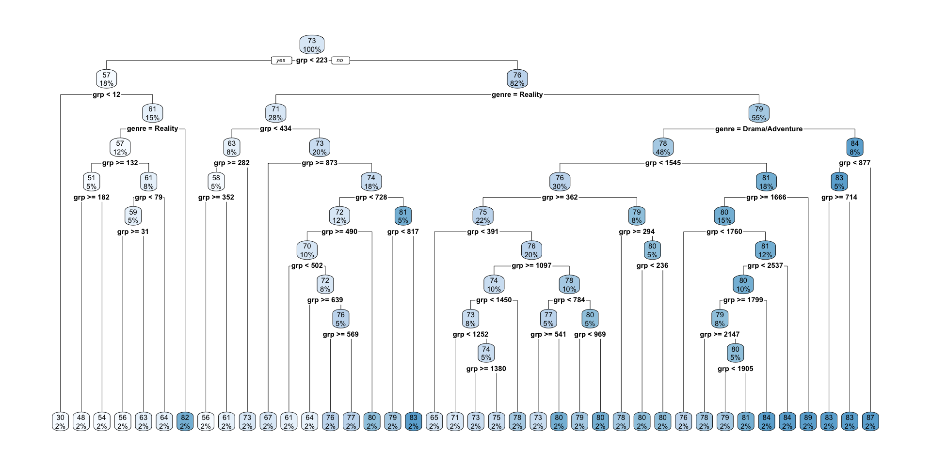
plotcp(full_nbc_tree)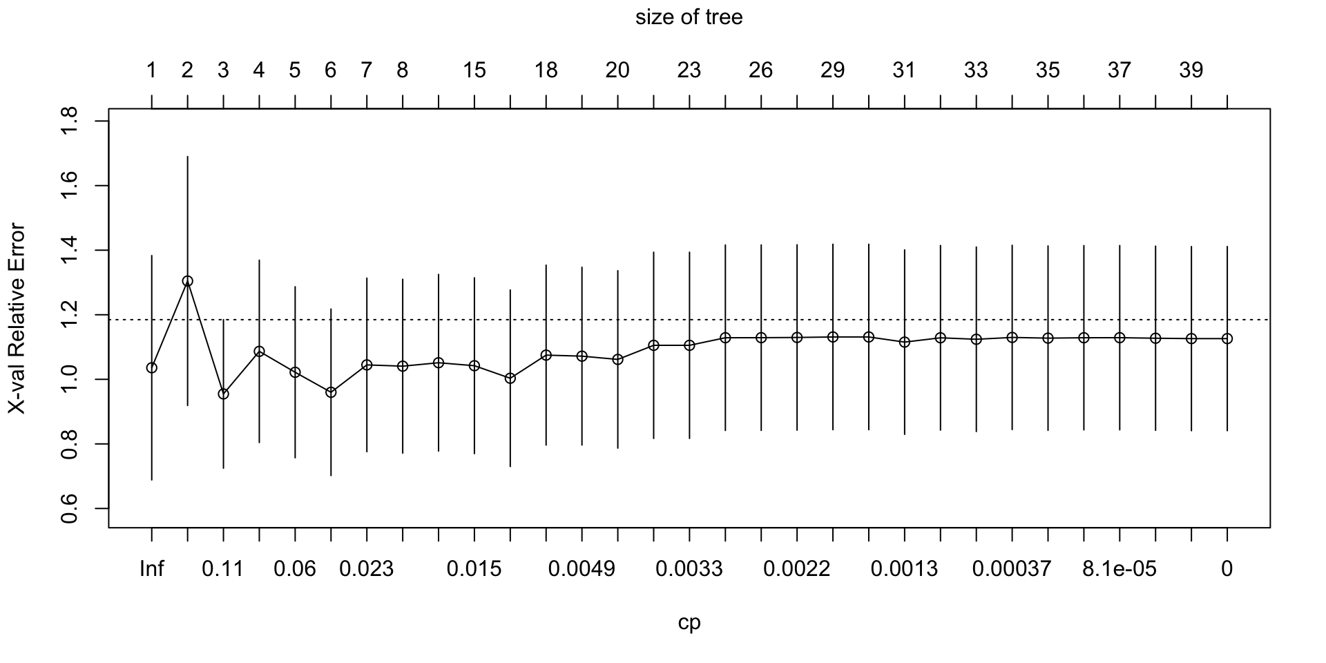
Variable Importance Plot
vip(full_nbc_tree, geom = "point")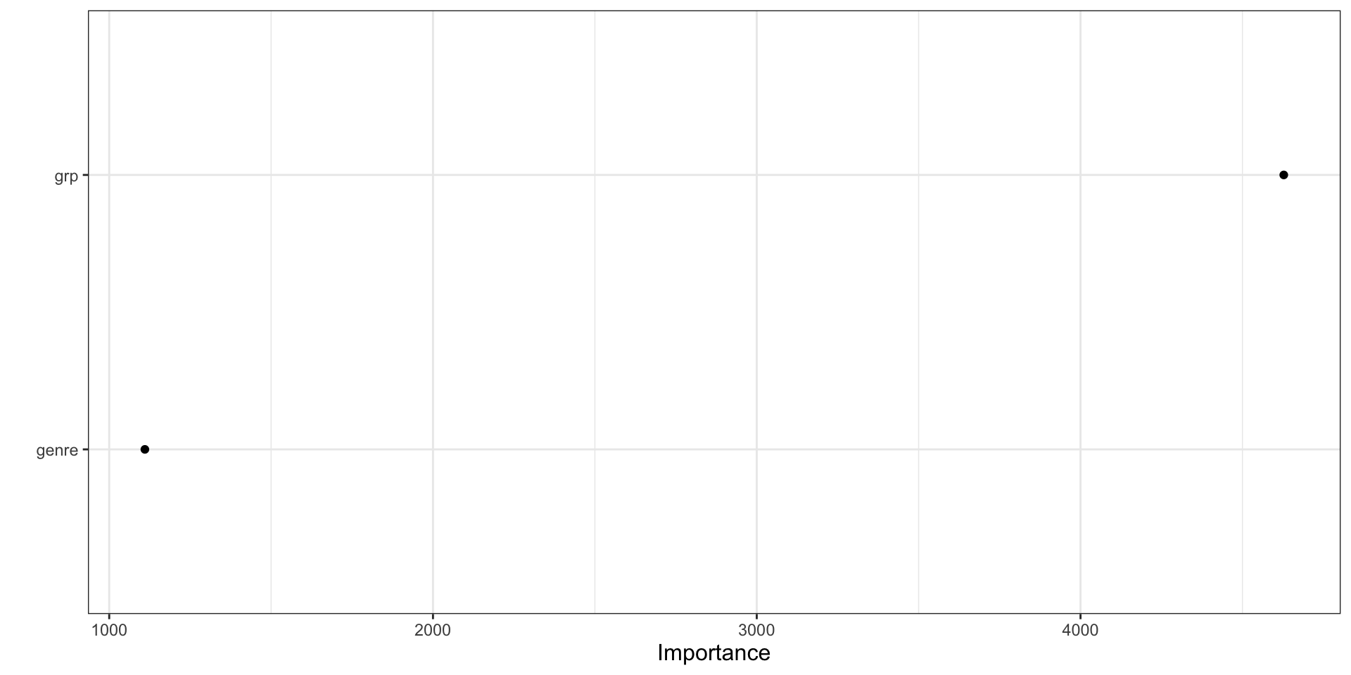
How to interpret vip() for a tree
- The plot ranks predictors by how much they contributed to improving the splits.
- Higher values mean the variable played a larger role in reducing node impurity.
- In a regression tree, this usually reflects reductions in squared-error loss.
- Variables near the top are more influential for prediction in this fitted model.
- Variable importance does not tell us the sign of the relationship.
What vip() does not tell us
- It does not say whether higher values of a predictor increase or decrease the outcome.
- It does not tell us whether the effect is linear, nonlinear, or highly interactive.
- It does not tell us whether the variable matters everywhere or only in a small part of the feature space.
- It should be treated as a ranking summary, not as a full interpretation on its own.
Partial Dependence Plot
# Partial Dependence for `grp`
partial(full_nbc_tree, pred.var = "grp") |>
  autoplot() +
  labs(title = "Partial Dependence of PE on GRP")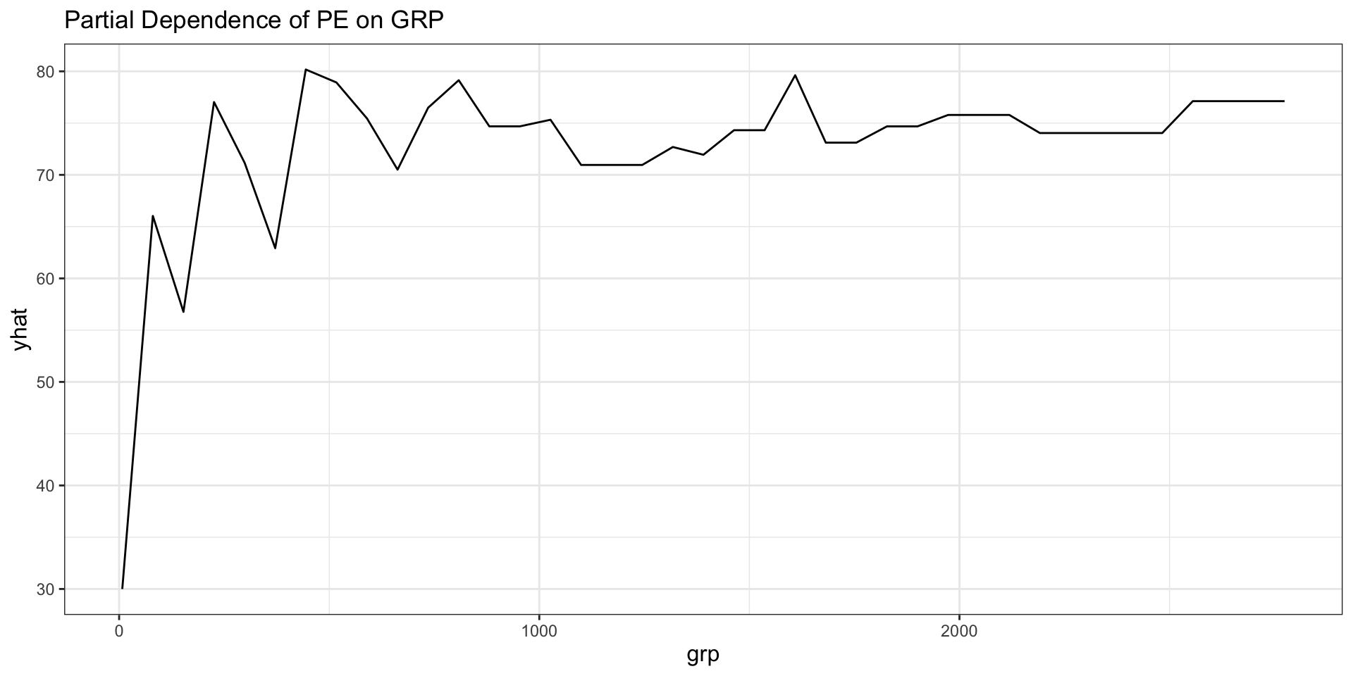
How to interpret pdp::partial()
- A partial dependence plot averages predictions over the observed values of all other predictors.
- The horizontal axis shows the focal predictor.
- The vertical axis shows the model’s average predicted outcome as that focal predictor changes.
- For trees, the plot often has a step-like appearance because tree predictions are piecewise constant.
- The PDP helps us see the direction and shape of the model-implied relationship.
Classification Tree
Classification goal
- Now predict
genrefrom audience demographics - This is a classification tree because the outcome is categorical
- The tree will try to create nodes that are relatively pure with respect to genre
Prepare data for the classification tree
nbc_genre <- nbc |>
  select(genre)
nbc_demog_only <- nbc_demog |>
  select(-show)

nbc_class_data <- bind_cols(
  nbc_genre,
  nbc_demog_only
)

paged_table(nbc_class_data)
Fit a larger classification tree
nbc_genre_tree_full <- rpart(
  genre ~ .,
  data = nbc_class_data,
  method = "class",
  control = rpart.control(cp = 0, minsplit = 2, minbucket = 1, xval = 10)
)

nbc_genre_tree_full
n= 40
node), split, n, loss, yval, (yprob)
* denotes terminal node
1) root 40 21 Drama/Adventure (0.47500000 0.42500000 0.10000000)
2) wired_cable_w_o_pay< 28.66505 22 6 Drama/Adventure (0.72727273 0.09090909 0.18181818)
4) vcr_owner>=83.749 17 1 Drama/Adventure (0.94117647 0.00000000 0.05882353)
8) territory_east_central< 16.45555 16 0 Drama/Adventure (1.00000000 0.00000000 0.00000000) *
9) territory_east_central>=16.45555 1 0 Situation Comedy (0.00000000 0.00000000 1.00000000) *
5) vcr_owner< 83.749 5 2 Situation Comedy (0.00000000 0.40000000 0.60000000)
10) territory_pacific>=18.87055 2 0 Reality (0.00000000 1.00000000 0.00000000) *
11) territory_pacific< 18.87055 3 0 Situation Comedy (0.00000000 0.00000000 1.00000000) *
3) wired_cable_w_o_pay>=28.66505 18 3 Reality (0.16666667 0.83333333 0.00000000)
6) black>=17.2017 3 0 Drama/Adventure (1.00000000 0.00000000 0.00000000) *
7) black< 17.2017 15 0 Reality (0.00000000 1.00000000 0.00000000) *ngives the number of observations in the node.lossis the number of observations that would be misclassified if we predicted the majority class for everyone in that node.yvalor the displayed the majority class of the node.yprobgives the estimated class probability for the predicted class.
How to interpret the fuller classification tree
rpart.plot(
  nbc_genre_tree_full,
  tweak = 0.8   # values greater than 1 make labels and boxes appear larger
                # values less than 1 make them smaller
)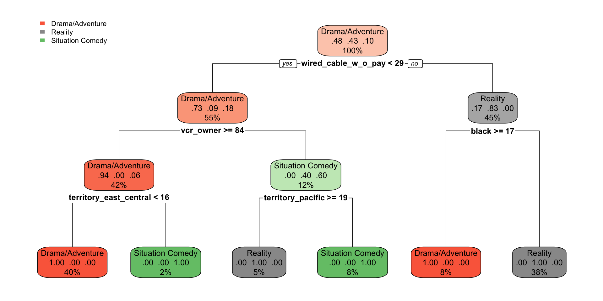
- Each split is chosen to make the child nodes more homogeneous by class.
- The label at the top of a node is the predicted class for that node.