library(tidyverse)
library(skimr)
library(janitor)
library(broom)
library(ggthemes)
library(rmarkdown)

library(rpart)
library(rpart.plot)
library(vip)
library(pdp)

theme_set(
  theme_bw() +
    theme(
      legend.position = "bottom",
      strip.background = element_rect(fill = "lightgray"),
      axis.title.x = element_text(size = rel(1.1)),
      axis.title.y = element_text(size = rel(1.1))
    )
)

scale_colour_discrete <- function(...) scale_color_colorblind(...)
scale_fill_discrete <- function(...) scale_fill_colorblind(...)Pruning Trees
MLB Data
Overview
In this lab, you will use decision trees to study two baseball-related prediction problems using Major League Baseball data.
You will do two tasks:
- Build a regression tree to predict
w_obausing batting statistics. - Build a classification tree to predict whether a batted ball becomes a home run.
Setup for Decision Trees
Part 1. Regression Tree with MLB Batting Data
Batting data
mlb_data <- read_csv(
  "http://bcdanl.github.io/data/mlb_fg_batting_2022.csv"
) |>
  clean_names() |>
  mutate(across(bb_percent:k_percent, readr::parse_number))

mlb_data |>
  paged_table()
What the variables mean
w_oba: weighted on-base average, a summary measure of offensive performancebb_percent: walk percentagek_percent: strikeout percentageiso: isolated poweravg: batting averageobp: on-base percentageslg: slugging percentagewar: wins above replacement
Step 2. Explore the variables
mlb_data |>
  select(w_oba, bb_percent, k_percent, iso) |>
skimr::skim()| Name | select(mlb_data, w_oba, b… |
| Number of rows | 157 |
| Number of columns | 4 |
| _______________________ | |
| Column type frequency: | |
| numeric | 4 |
| ________________________ | |
| Group variables | None |
Variable type: numeric
| skim_variable | n_missing | complete_rate | mean | sd | p0 | p25 | p50 | p75 | p100 | hist |
|---|---|---|---|---|---|---|---|---|---|---|
| w_oba | 0 | 1 | 0.33 | 0.04 | 0.25 | 0.31 | 0.33 | 0.35 | 0.44 | ▃▇▇▃▁ |
| bb_percent | 0 | 1 | 8.80 | 2.97 | 3.50 | 6.50 | 8.60 | 11.00 | 20.30 | ▆▇▆▁▁ |
| k_percent | 0 | 1 | 20.47 | 5.89 | 8.10 | 16.10 | 19.90 | 24.80 | 36.10 | ▃▇▇▅▁ |
| iso | 0 | 1 | 0.17 | 0.06 | 0.05 | 0.12 | 0.17 | 0.20 | 0.35 | ▃▇▇▂▁ |
mlb_data |>
  ggplot(aes(x = iso, y = w_oba)) +
  geom_point(alpha = 0.6) +
  labs(
    title = "wOBA and ISO",
    x = "ISO",
    y = "wOBA"
  )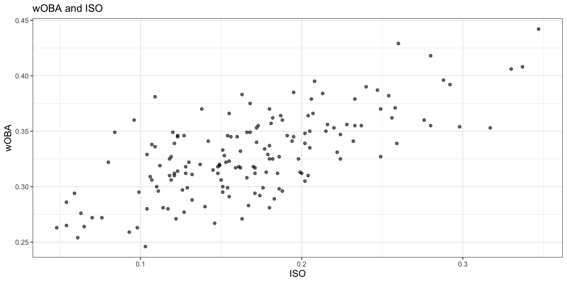
Task 1
Write 2 to 3 sentences describing the relationship between iso and w_oba. What pattern do you see in the scatterplot?
Answer:
There is a clear positive relationship between iso and w_oba. Players with higher isolated power tend to have higher offensive production overall, so the cloud of points slopes upward. The pattern is not perfectly linear, but stronger power clearly tends to be associated with a larger w_oba.
Step 3. Fit an initial regression tree
We will begin with a simple decision tree using three predictors.
mlb_tree_1 <- rpart(
  w_oba ~ bb_percent + k_percent + iso,
  data = mlb_data,
  method = "anova"
)

mlb_tree_1
n= 157
node), split, n, deviance, yval
* denotes terminal node
1) root 157 0.215948200 0.3291338
2) iso< 0.2055 123 0.113126200 0.3175691
4) iso< 0.1035 16 0.016633000 0.2837500 *
5) iso>=0.1035 107 0.075457050 0.3226262
10) bb_percent< 8.75 65 0.039689380 0.3146154
20) k_percent>=27.15 9 0.001585556 0.2902222 *
21) k_percent< 27.15 56 0.031887930 0.3185357
42) iso< 0.152 27 0.010937850 0.3089259 *
43) iso>=0.152 29 0.016135240 0.3274828
86) k_percent>=21.85 17 0.008568235 0.3194706 *
87) k_percent< 21.85 12 0.004929667 0.3388333 *
11) bb_percent>=8.75 42 0.025140980 0.3350238
22) k_percent>=23.45 11 0.002378909 0.3129091 *
23) k_percent< 23.45 31 0.015473480 0.3428710
46) iso< 0.159 15 0.006778000 0.3320000 *
47) iso>=0.159 16 0.005260937 0.3530625 *
3) iso>=0.2055 34 0.026860970 0.3709706
6) iso< 0.2595 23 0.009236609 0.3608696 *
7) iso>=0.2595 11 0.010370910 0.3920909 *rpart.plot(mlb_tree_1)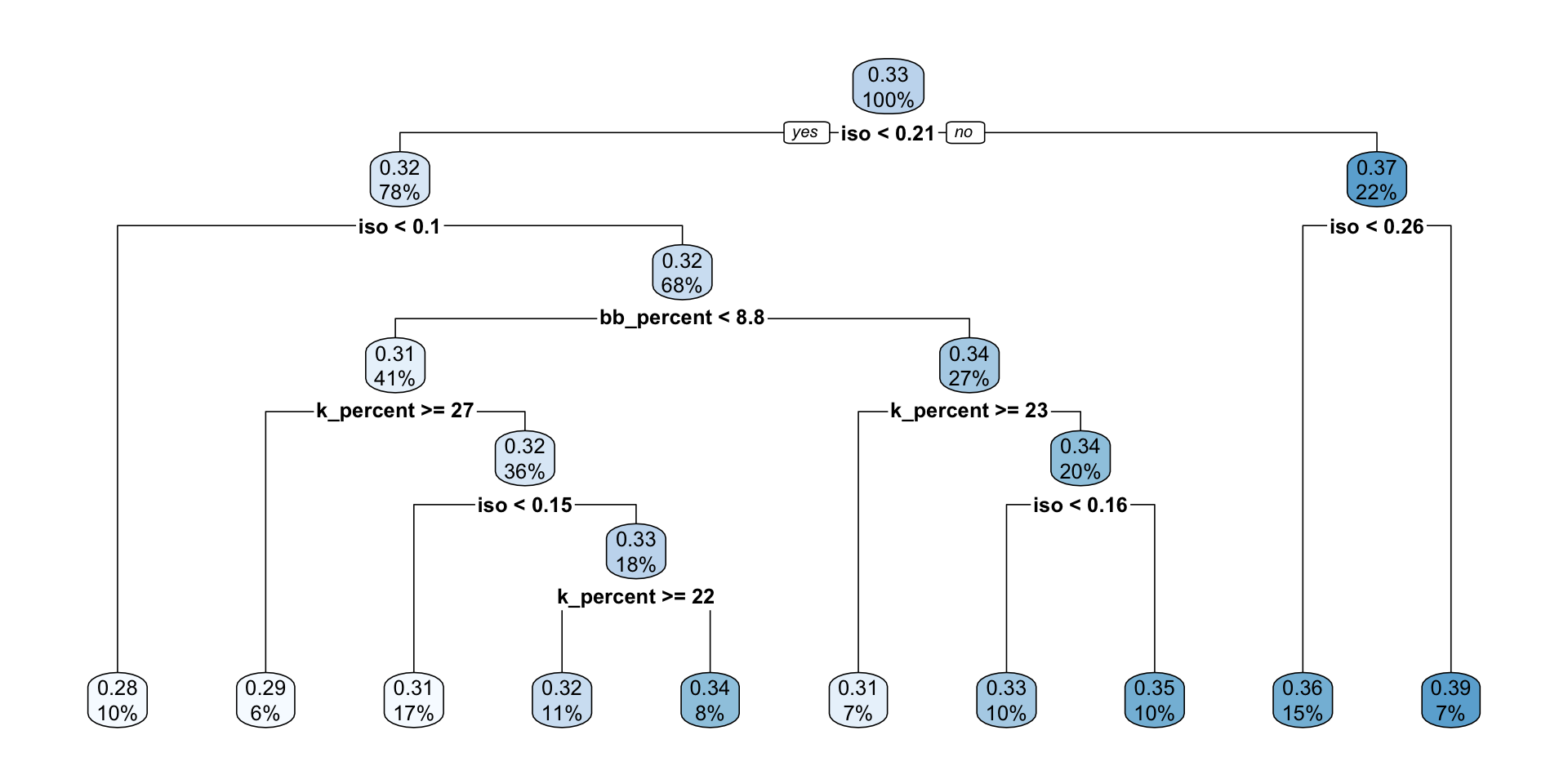
Task 2
Answer the following in complete sentences:
- Which variable appears at the first split?
- What does that suggest about the predictor’s importance in this tree?
- Choose one terminal node and explain what its predicted value means.
Answer:
- The first split is on
iso. - This suggests that
isois the most important predictor near the top of this tree because it gives the largest reduction in impurity at the first decision point. - For example, if a terminal node predicts a
w_obaaround 0.37, that means players whose statistics place them in that region of the tree are predicted to have an averagew_obaof about 0.37.
Step 4. Grow a larger tree
Now let the algorithm grow a much more flexible tree.
mlb_tree_full <- rpart(
  w_oba ~ bb_percent + k_percent + iso,
  data = mlb_data,
  method = "anova",
  control = rpart.control(cp = 0, xval = 10)
)

mlb_tree_full
n= 157
node), split, n, deviance, yval
* denotes terminal node
1) root 157 0.215948200 0.3291338
2) iso< 0.2055 123 0.113126200 0.3175691
4) iso< 0.1035 16 0.016633000 0.2837500 *
5) iso>=0.1035 107 0.075457050 0.3226262
10) bb_percent< 8.75 65 0.039689380 0.3146154
20) k_percent>=27.15 9 0.001585556 0.2902222 *
21) k_percent< 27.15 56 0.031887930 0.3185357
42) iso< 0.152 27 0.010937850 0.3089259
84) k_percent>=18.5 10 0.003274000 0.3020000 *
85) k_percent< 18.5 17 0.006902000 0.3130000 *
43) iso>=0.152 29 0.016135240 0.3274828
86) k_percent>=21.85 17 0.008568235 0.3194706 *
87) k_percent< 21.85 12 0.004929667 0.3388333 *
11) bb_percent>=8.75 42 0.025140980 0.3350238
22) k_percent>=23.45 11 0.002378909 0.3129091 *
23) k_percent< 23.45 31 0.015473480 0.3428710
46) iso< 0.159 15 0.006778000 0.3320000 *
47) iso>=0.159 16 0.005260937 0.3530625 *
3) iso>=0.2055 34 0.026860970 0.3709706
6) iso< 0.2595 23 0.009236609 0.3608696
12) k_percent>=18.8 13 0.004075077 0.3523846 *
13) k_percent< 18.8 10 0.003008900 0.3719000 *
7) iso>=0.2595 11 0.010370910 0.3920909 *rpart.plot(mlb_tree_full)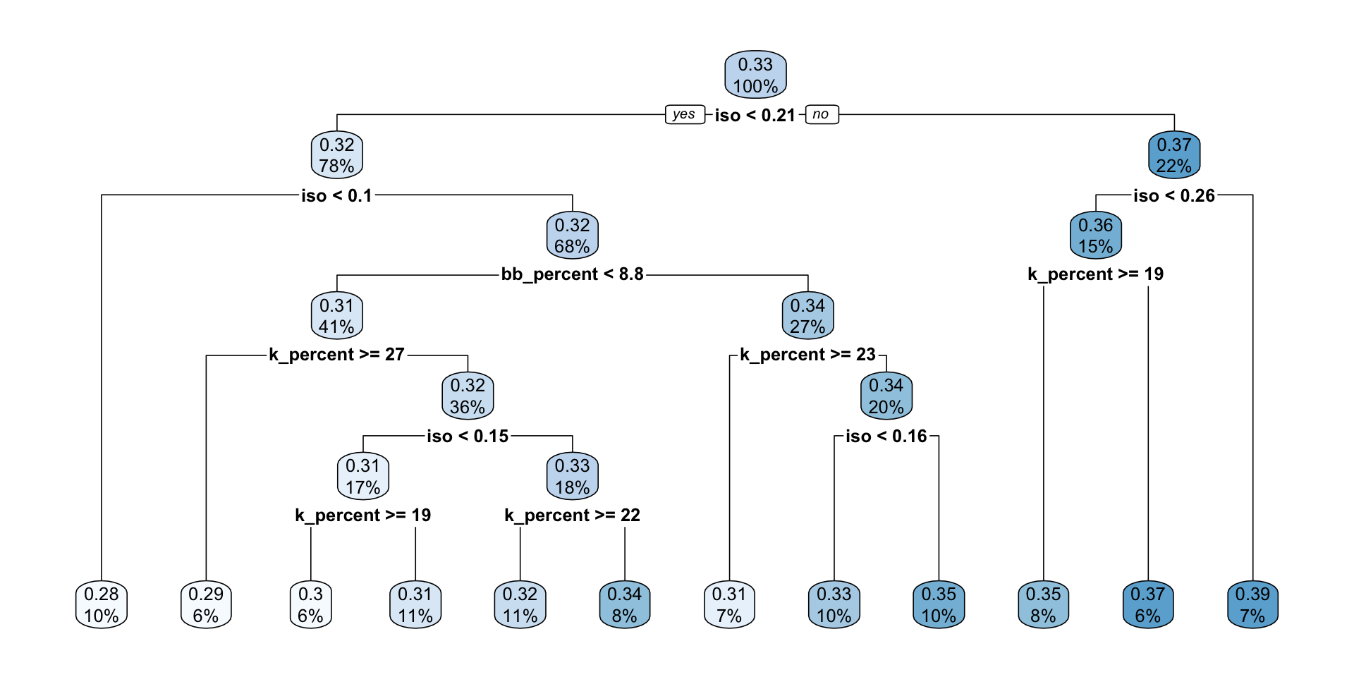
plotcp(mlb_tree_full)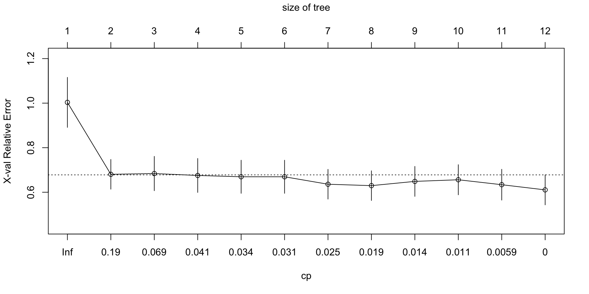
Task 3
Answer the following:
- Compared with the first tree, is this tree more or less complex?
- Why might a very large tree be a problem for out-of-sample prediction?
- Looking at
plotcp(), what kind of tree are we usually trying to choose: the biggest tree, the smallest tree, or a tree that balances fit and complexity?
Answer:
- This tree is more complex than the first tree because it has more splits and more terminal nodes.
- A very large tree can overfit the training data by capturing noise or very specific local patterns that do not generalize well to new observations.
- We usually want a tree that balances fit and complexity rather than simply choosing the biggest or smallest tree.
Step 5. Fine-tune tree growth before pruning
Before pruning, try a few different tree-growth settings. This is a simple form of hyperparameter tuning. The goal is to see how choices like minsplit and maxdepth affect the size of the tree and the cross-validated error.
reg_tuning_grid <- tribble(
  ~minsplit, ~maxdepth,
  20,        4,
  20,        6,
  30,        4,
  30,        6,
  40,        4,
  40,        6
)

reg_tuning_results <- reg_tuning_grid

fit_list <- vector("list", nrow(reg_tuning_results))
cp_table_list <- vector("list", nrow(reg_tuning_results))
min_xerror_vec <- numeric(nrow(reg_tuning_results))
best_cp_vec <- numeric(nrow(reg_tuning_results))
nsplit_at_best_cp_vec <- numeric(nrow(reg_tuning_results))

for (i in seq_len(nrow(reg_tuning_results))) {

  fit_list[[i]] <- rpart(
    w_oba ~ bb_percent + k_percent + iso,
    data = mlb_data,
    method = "anova",
    control = rpart.control(
      cp = 0,
      xval = 10,
      minsplit = reg_tuning_results$minsplit[i],
      maxdepth = reg_tuning_results$maxdepth[i]
    )
  )

  cp_table_list[[i]] <- as_tibble(fit_list[[i]]$cptable)

  min_xerror_vec[i] <- min(cp_table_list[[i]]$xerror)

  best_cp_vec[i] <- cp_table_list[[i]] |>
    slice_min(xerror, n = 1) |>
    pull(CP)

  nsplit_at_best_cp_vec[i] <- cp_table_list[[i]] |>
    filter(CP == best_cp_vec[i]) |>
    slice(1) |>
    pull(nsplit)
}

reg_tuning_results <- reg_tuning_results |>
  mutate(
    fit = fit_list,
    cp_table = cp_table_list,
    min_xerror = min_xerror_vec,
    best_cp = best_cp_vec,
    nsplit_at_best_cp = nsplit_at_best_cp_vec
  ) |>
  select(minsplit, maxdepth, min_xerror, best_cp, nsplit_at_best_cp)

reg_tuning_results |>
  paged_table()
Task 4
Answer the following:
- Which combination of
minsplitandmaxdepthgives the smallest cross-validated error? - Does a deeper tree always give the best
xerror? - Based on this table, which setting would you carry forward to pruning, and why?
Answer:
- In this setup,
minsplit = 20andmaxdepth = 6tends to give the smallest cross-validated error. - No. A deeper tree does not always give the best
xerrorbecause extra depth can improve fit in-sample while hurting generalization. - I would carry forward
minsplit = 20andmaxdepth = 6because it gives the best or near-best cross-validated performance while still being reasonably interpretable.
Step 6. Find the best complexity parameter for your tuned tree
Use the hyperparameter setting you prefer from Step 5. In the example below, we use minsplit = 20 and maxdepth = 6. You may change these values if your preferred setting is different.
mlb_tree_tuned <- rpart(
  w_oba ~ bb_percent + k_percent + iso,
  data = mlb_data,
  method = "anova",
  control = rpart.control(cp = 0, xval = 10, minsplit = 30, maxdepth = 6)
)

plotcp(mlb_tree_tuned)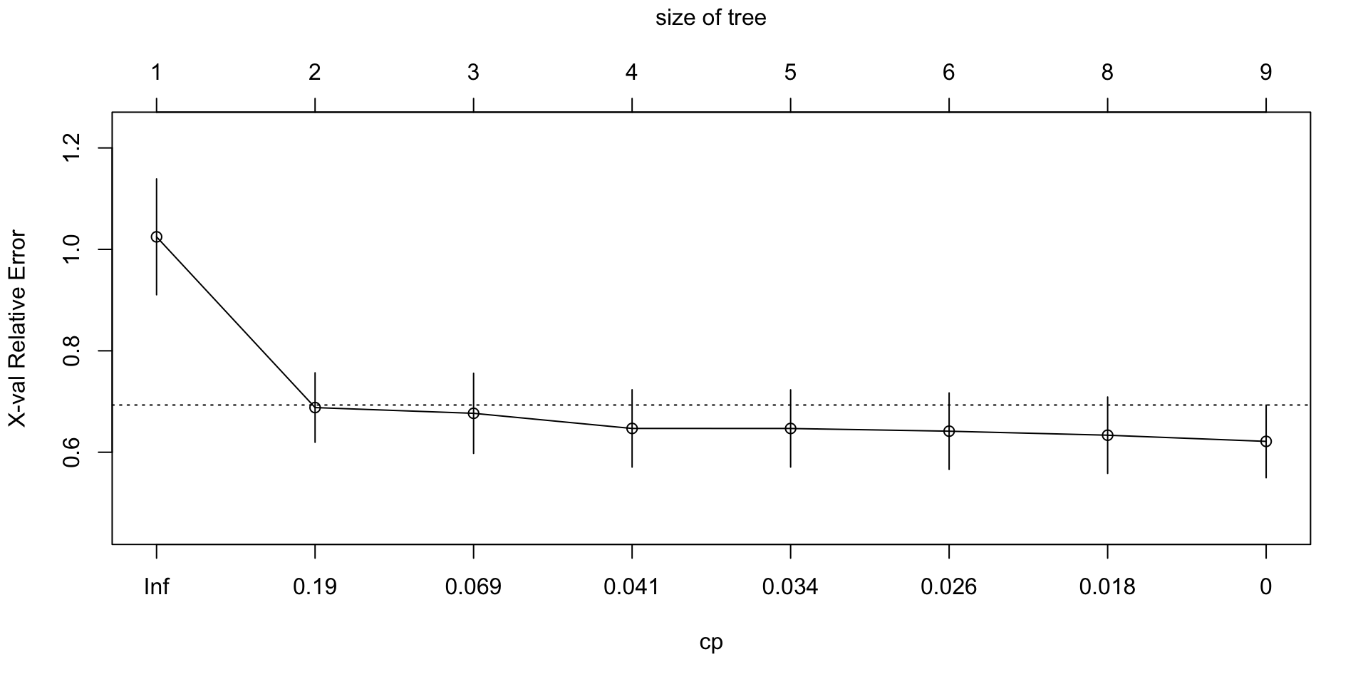
cp_table <- as_tibble(mlb_tree_tuned$cptable)

cp_table |>
  paged_table()
best_cp <- cp_table |>
slice_min(xerror, n = 1) |>
pull(CP)
best_cp[1] 0Task 5
What does the xerror column represent? Why do we often use it when choosing the pruning parameter?
Answer:
The xerror column reports the cross-validated prediction error relative to the root node benchmark. We use it to choose the pruning parameter because it gives a better sense of out-of-sample performance than training error alone.
Step 7. Prune the tuned tree
mlb_tree_pruned <- prune(mlb_tree_tuned, cp = best_cp)

mlb_tree_pruned
n= 157
node), split, n, deviance, yval
* denotes terminal node
1) root 157 0.215948200 0.3291338
2) iso< 0.2055 123 0.113126200 0.3175691
4) iso< 0.1035 16 0.016633000 0.2837500 *
5) iso>=0.1035 107 0.075457050 0.3226262
10) bb_percent< 8.75 65 0.039689380 0.3146154
20) k_percent>=26.55 10 0.004590000 0.2960000 *
21) k_percent< 26.55 55 0.031004000 0.3180000
42) iso< 0.152 27 0.010937850 0.3089259 *
43) iso>=0.152 28 0.015699250 0.3267500 *
11) bb_percent>=8.75 42 0.025140980 0.3350238
22) k_percent>=23.45 11 0.002378909 0.3129091 *
23) k_percent< 23.45 31 0.015473480 0.3428710
46) iso< 0.159 15 0.006778000 0.3320000 *
47) iso>=0.159 16 0.005260937 0.3530625 *
3) iso>=0.2055 34 0.026860970 0.3709706
6) iso< 0.2595 23 0.009236609 0.3608696 *
7) iso>=0.2595 11 0.010370910 0.3920909 *rpart.plot(mlb_tree_pruned)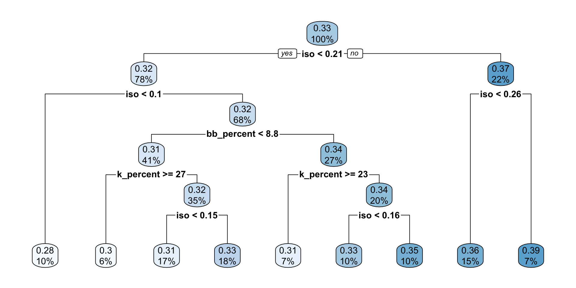
print(mlb_tree_tuned$cptable, digits = 10) CP nsplit rel error xerror xstd
1 0.35175593513 0 1.0000000000 1.0115094961 0.11255597744
2 0.09741279039 1 0.6482440649 0.7096175788 0.06879068064
3 0.04920942319 2 0.5508312745 0.7037890786 0.07592084735
4 0.03375153638 3 0.5016218513 0.6240138680 0.06755193279
5 0.03358885650 4 0.4678703149 0.6331998564 0.06680105435
6 0.01959331708 5 0.4342814584 0.6179095448 0.06409298010
7 0.01590449243 7 0.3950948242 0.6099371376 0.06346946803
8 0.00000000000 8 0.3791903318 0.5929039991 0.06079484965print(mlb_tree_full$cptable, digits = 10) CP nsplit rel error xerror xstd
1 0.351755935125 0 1.0000000000 1.0186184109 0.11349670591
2 0.097412790388 1 0.6482440649 0.7196312849 0.06943743859
3 0.049209423195 2 0.5508312745 0.7372628885 0.08074439379
4 0.033751536385 3 0.5016218513 0.6910032710 0.07802543374
5 0.033588856500 4 0.4678703149 0.7012482373 0.07923813434
6 0.028784221147 5 0.4342814584 0.6593713603 0.07467891204
7 0.022296252245 6 0.4054972373 0.6198535930 0.07212207274
8 0.015904492433 7 0.3832009850 0.6294197359 0.07081025629
9 0.012212834038 8 0.3672964926 0.6467733344 0.07523410710
10 0.009968278788 9 0.3550836585 0.6251411086 0.07419204274
11 0.003527938104 10 0.3451153798 0.6127933806 0.07314836497
12 0.000000000000 11 0.3415874417 0.6191285627 0.07354980500Task 6
Compare the tuned unpruned tree and the pruned tree.
Write 2 to 4 sentences addressing these questions:
- What became simpler after pruning?
- Why can a pruned tree sometimes predict better on new data even if it fits the training data less closely?
- Did your earlier hyperparameter choices seem to matter for the final pruned result?
Answer:
After pruning, the tree has fewer splits and fewer terminal nodes, so the model is easier to explain. A pruned tree can predict better on new data because it removes weaker splits that may mainly capture noise in the training sample. The earlier hyperparameter choices still matter because they affect the size and shape of the tree before pruning, which changes what pruning is able to keep or remove.
Part 2. Classification Tree with MLB Batted-Ball Data
Batted-ball data
batted_ball_data <- read_csv(
  "http://bcdanl.github.io/data/mlb_batted_balls_2022.csv"
) |>
  mutate(is_hr = as.factor(events == "home_run")) |>
  filter(
    !is.na(launch_angle),
    !is.na(launch_speed),
    !is.na(is_hr)
  )

batted_ball_data |>
  paged_table()
batted_ball_data |>
count(is_hr)# A tibble: 2 × 2
is_hr n
<fct> <int>
1 FALSE 6702
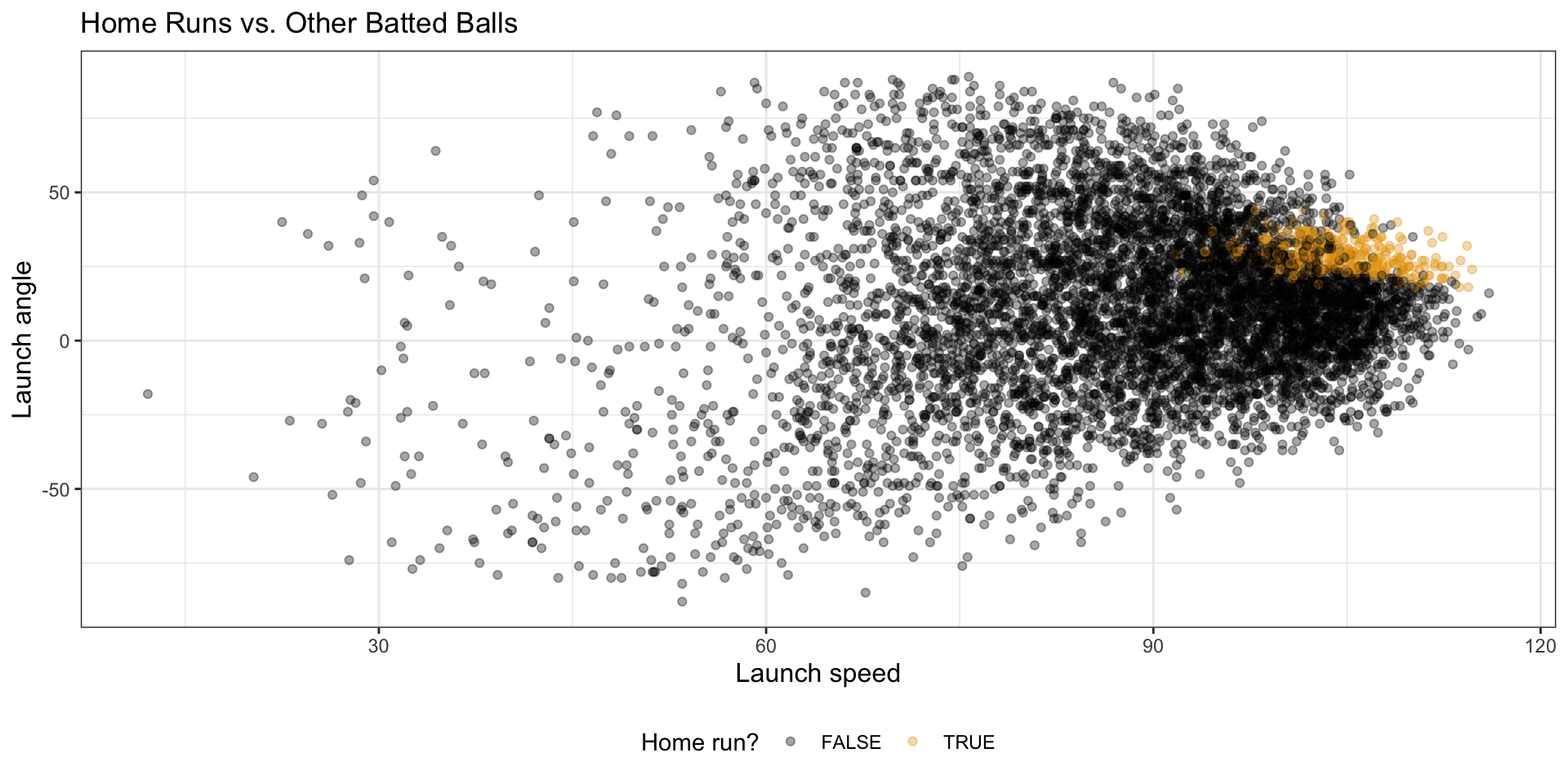
2 TRUE 333Visualize the classification problem
batted_ball_data |>
  ggplot(aes(x = launch_speed, y = launch_angle, color = is_hr)) +
  geom_point(alpha = 0.35) +
  labs(
    title = "Home Runs vs. Other Batted Balls",
    x = "Launch speed",
    y = "Launch angle",
    color = "Home run?"
  )
Under construction