library(tidyverse)
library(factoextra)
library(cluster)
library(fpc)
library(skimr)

wine <- read_csv("https://bcdanl.github.io/data/wine_data.csv")K-means Clustering and PCA
Wine Data
Data
Variable Description
| Variable | Description |
|---|---|
acidity_fixed |
Fixed acidity in the wine. |
acidity_volatile |
Volatile acidity in the wine. |
acidity_citric |
Amount of citric acid in the wine. |
residual_sugar |
Residual sugar remaining after fermentation. |
chlorides |
Amount of chlorides in the wine. |
so2_free |
Free sulfur dioxide concentration. |
so2_tot |
Total sulfur dioxide concentration. |
density |
Density of the wine. |
pH |
pH level of the wine. |
so4_2 |
Sulfate concentration. |
alcohol |
Alcohol content of the wine. |
quality |
Wine quality score. |
color |
Wine type: red or white. |
Question 1. Inspect the data
wine |>
skim()| Name | wine |
| Number of rows | 6497 |
| Number of columns | 13 |
| _______________________ | |
| Column type frequency: | |
| character | 1 |
| numeric | 12 |
| ________________________ | |
| Group variables | None |
Variable type: character
| skim_variable | n_missing | complete_rate | min | max | empty | n_unique | whitespace |
|---|---|---|---|---|---|---|---|
| color | 0 | 1 | 3 | 5 | 0 | 2 | 0 |
Variable type: numeric
| skim_variable | n_missing | complete_rate | mean | sd | p0 | p25 | p50 | p75 | p100 | hist |
|---|---|---|---|---|---|---|---|---|---|---|
| acidity_fixed | 0 | 1 | 7.22 | 1.30 | 3.80 | 6.40 | 7.00 | 7.70 | 15.90 | ▂▇▁▁▁ |
| acidity_volatile | 0 | 1 | 0.34 | 0.16 | 0.08 | 0.23 | 0.29 | 0.40 | 1.58 | ▇▂▁▁▁ |
| acidity_citric | 0 | 1 | 0.32 | 0.15 | 0.00 | 0.25 | 0.31 | 0.39 | 1.66 | ▇▅▁▁▁ |
| residual_sugar | 0 | 1 | 5.44 | 4.76 | 0.60 | 1.80 | 3.00 | 8.10 | 65.80 | ▇▁▁▁▁ |
| chlorides | 0 | 1 | 0.06 | 0.04 | 0.01 | 0.04 | 0.05 | 0.06 | 0.61 | ▇▁▁▁▁ |
| so2_free | 0 | 1 | 30.53 | 17.75 | 1.00 | 17.00 | 29.00 | 41.00 | 289.00 | ▇▁▁▁▁ |
| so2_tot | 0 | 1 | 115.74 | 56.52 | 6.00 | 77.00 | 118.00 | 156.00 | 440.00 | ▅▇▂▁▁ |
| density | 0 | 1 | 0.99 | 0.00 | 0.99 | 0.99 | 0.99 | 1.00 | 1.04 | ▇▂▁▁▁ |
| pH | 0 | 1 | 3.22 | 0.16 | 2.72 | 3.11 | 3.21 | 3.32 | 4.01 | ▁▇▆▁▁ |
| so4_2 | 0 | 1 | 0.53 | 0.15 | 0.22 | 0.43 | 0.51 | 0.60 | 2.00 | ▇▃▁▁▁ |
| alcohol | 0 | 1 | 10.49 | 1.19 | 8.00 | 9.50 | 10.30 | 11.30 | 14.90 | ▃▇▅▂▁ |
| quality | 0 | 1 | 5.82 | 0.87 | 3.00 | 5.00 | 6.00 | 6.00 | 9.00 | ▁▆▇▃▁ |
Answer:
The data set contains wine observations with chemical measurements, a quality score, and a color variable. Most variables are numeric chemical variables, while color is categorical. The variables quality and color should not be used directly for unsupervised clustering because quality is an outcome-type rating and color is a known label. For clustering, we want the algorithm to discover patterns from the chemical variables only.
Question 2. Create a cleaned analysis data set
wine_clust <- wine |>
  select(-quality, -color)

wine_scaled <- wine_clust |>
  scale()

dim(wine_scaled)
[1] 6497 11wine_scaled |>
as_tibble() |>
summarise(across(everything(), list(mean = mean, sd = sd)))# A tibble: 1 × 22
acidity_fixed_mean acidity_fixed_sd acidity_volatile_mean acidity_volatile_sd
<dbl> <dbl> <dbl> <dbl>
1 1.39e-15 1.00 -2.72e-14 1.00
# ℹ 18 more variables: acidity_citric_mean <dbl>, acidity_citric_sd <dbl>,
# residual_sugar_mean <dbl>, residual_sugar_sd <dbl>, chlorides_mean <dbl>,
# chlorides_sd <dbl>, so2_free_mean <dbl>, so2_free_sd <dbl>,
# so2_tot_mean <dbl>, so2_tot_sd <dbl>, density_mean <dbl>, density_sd <dbl>,
# pH_mean <dbl>, pH_sd <dbl>, so4_2_mean <dbl>, so4_2_sd <dbl>,
# alcohol_mean <dbl>, alcohol_sd <dbl>Answer:
The cleaned analysis data set removes quality and color, leaving only the numeric chemical variables. Scaling is important because k-means is based on distance. If variables are not scaled, variables measured on larger scales, such as total sulfur dioxide, can dominate variables measured on smaller scales, such as pH or density. After scaling, each variable has mean 0 and standard deviation 1, so the clustering algorithm treats the variables more comparably.
Question 3. Fit a k-means model with 2 clusters
set.seed(320)

km2 <- kmeans(wine_scaled, centers = 2, nstart = 25)km2$size[1] 1643 4854km2$centers acidity_fixed acidity_volatile acidity_citric residual_sugar chlorides
1 0.8286464 1.1678795 -0.3378091 -0.5903919 0.9216848
2 -0.2804833 -0.3953082 0.1143429 0.1998380 -0.3119753
so2_free so2_tot density pH so4_2 alcohol
1 -0.8316090 -1.1872380 0.6815493 0.5673286 0.8430523 -0.07569241
2 0.2814861 0.4018607 -0.2306934 -0.1920315 -0.2853595 0.02562065km_centers <- km2$centers |>
as_tibble() |>
t() |>
as.data.frame() |>
mutate(diff = V2 - V1) |>
arrange(-abs(diff))
km_centers V1 V2 diff
so2_tot -1.18723795 0.40186072 1.5890987
acidity_volatile 1.16787955 -0.39530822 -1.5631878
chlorides 0.92168475 -0.31197529 -1.2336600
so4_2 0.84305233 -0.28535949 -1.1284118
so2_free -0.83160895 0.28148610 1.1130951
acidity_fixed 0.82864638 -0.28048331 -1.1091297
density 0.68154931 -0.23069335 -0.9122427
residual_sugar -0.59039189 0.19983805 0.7902299
pH 0.56732860 -0.19203150 -0.7593601
acidity_citric -0.33780910 0.11434288 0.4521520
alcohol -0.07569241 0.02562065 0.1013131Answer:
The cluster sizes show how many wines were assigned to each of the two groups. The cluster centers are reported in standardized units, so positive values mean that the cluster is above the overall average for that variable and negative values mean that the cluster is below the overall average. The variables with the largest absolute differences in km_centers are the most useful for distinguishing the two clusters. In this data set, variables such as total sulfur dioxide, volatile acidity, residual sugar, alcohol, and density are likely to be important for separating the clusters.
Question 4. Add the cluster labels back to the data and profile the clusters
length(km2$cluster)[1] 6497wine_km <- wine |>
mutate(cluster = km2$cluster)wine_km |>
group_by(cluster) |>
summarise(
n = n(),
alcohol = mean(alcohol),
acidity_volatile = mean(acidity_volatile),
residual_sugar = mean(residual_sugar),
so2_tot = mean(so2_tot),
quality = mean(quality),
.groups = "drop"
)# A tibble: 2 × 7
cluster n alcohol acidity_volatile residual_sugar so2_tot quality
<int> <int> <dbl> <dbl> <dbl> <dbl> <dbl>
1 1 1643 10.4 0.532 2.63 48.6 5.60
2 2 4854 10.5 0.275 6.39 138. 5.89Answer:
This summary table profiles the two clusters using variables that are easy to interpret. One cluster tends to have higher values for some chemical characteristics, while the other cluster tends to have lower values. Comparing alcohol, acidity_volatile, residual_sugar, and so2_tot helps describe what the clusters mean substantively. The average quality score is included only after clustering so that we can compare the clusters, not because quality was used to create the clusters.
Question 5. Compare cluster membership with wine color
wine_km |>
  count(color, cluster) |>
  group_by(color) |>
  mutate(pct = n / sum(n)) |>
  ungroup()
# A tibble: 4 × 4
color cluster n pct
<chr> <int> <int> <dbl>
1 red 1 1575 0.985
2 red 2 24 0.0150
3 white 1 68 0.0139
4 white 2 4830 0.986 wine_km |>
count(cluster, color) |>
group_by(cluster) |>
mutate(pct = n / sum(n)) |>
ungroup()# A tibble: 4 × 4
cluster color n pct
<int> <chr> <int> <dbl>
1 1 red 1575 0.959
2 1 white 68 0.0414
3 2 red 24 0.00494
4 2 white 4830 0.995 Answer:
Cluster membership appears to be strongly related to wine color. This suggests that the chemical variables contain enough information for k-means to recover a grouping that looks similar to red versus white wine, even though the color variable was not included in the clustering model. This is interesting because it shows the logic of unsupervised learning: the algorithm did not receive the true label, but it still found structure in the data that corresponds to a meaningful real-world category.
Question 6. Make one simple scatter plot
wine_km |>
ggplot(aes(x = so2_tot,
y = acidity_volatile,
color = factor(cluster))) +
geom_point(alpha = 0.2) +
labs(
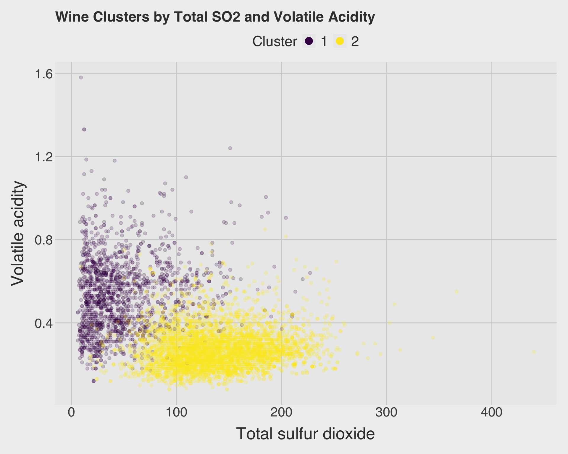
title = "Wine Clusters by Total SO2 and Volatile Acidity",
x = "Total sulfur dioxide",
y = "Volatile acidity",
color = "Cluster"
) +
guides(
color = guide_legend(override.aes = list(alpha = 1, size = 4))
)
Answer:
The scatter plot shows some visible separation between the two clusters, especially because total sulfur dioxide and volatile acidity are chemically meaningful variables. However, there is still overlap. This is expected because k-means used all scaled chemical variables together, while a two-dimensional scatter plot only shows two variables at a time. Wines that overlap in this two-variable plot may still differ on other variables used by the clustering algorithm.
Question 7. Try several values of \(k\)
km2$tot.withinss[1] 56135.28set.seed(320)
km3 <- kmeans(wine_scaled, centers = 3, nstart = 25)
km4 <- kmeans(wine_scaled, centers = 4, nstart = 25)
km5 <- kmeans(wine_scaled, centers = 5, nstart = 25)
km6 <- kmeans(wine_scaled, centers = 6, nstart = 25)
tot.withinss <- c(
"km2" = km2$tot.withinss,
"km3" = km3$tot.withinss,
"km4" = km4$tot.withinss,
"km5" = km5$tot.withinss,
"km6" = km6$tot.withinss
)
tot.withinss km2 km3 km4 km5 km6
56135.28 45569.97 40714.72 38063.17 36263.75 which.min(tot.withinss)km6
5 tibble(
k = 2:6,
total_withinss = tot.withinss
) |>
ggplot(aes(x = k, y = total_withinss)) +
geom_line() +
geom_point(size = 3) +
labs(
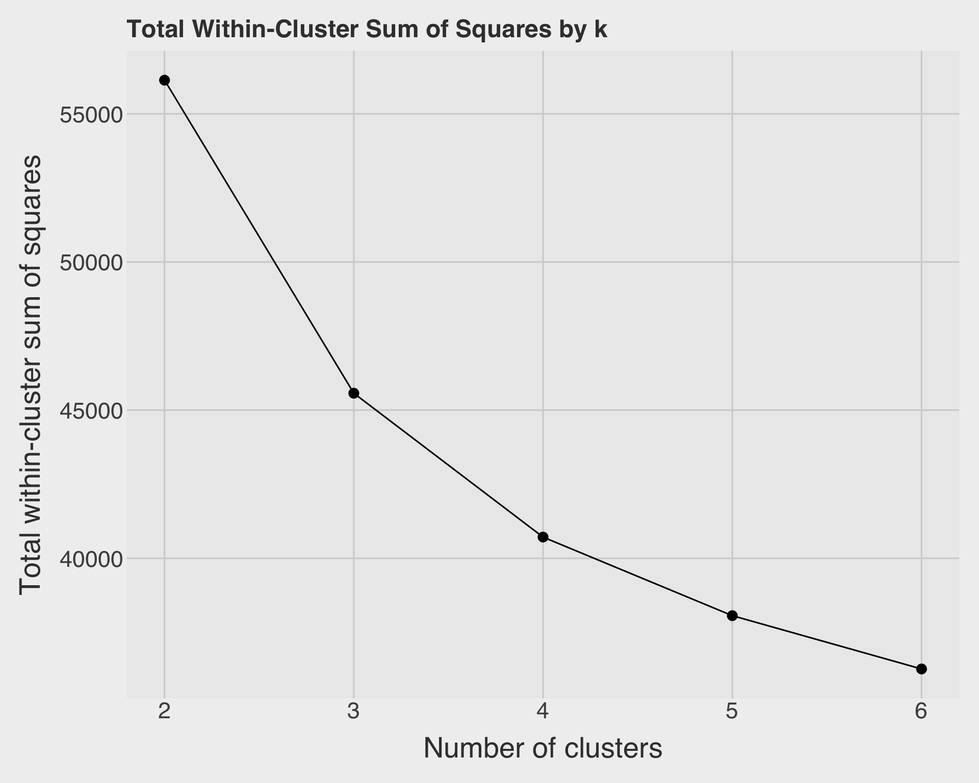
title = "Total Within-Cluster Sum of Squares by k",
x = "Number of clusters",
y = "Total within-cluster sum of squares"
)
set.seed(320)
clustering_ch  <- kmeansruns(wine_scaled, krange = 2:6, criterion = "ch")
clustering_asw <- kmeansruns(wine_scaled, krange = 2:6, criterion = "asw")

clustering_ch$bestk   # best k by Calinski-Harabasz
[1] 3clustering_asw$bestk # best k by Average Silhouette Width[1] 2set.seed(320)
fviz_nbclust(wine_scaled,
FUNcluster = kmeans,
method = "wss",
k.max = 10) +
labs(title = "Elbow Method — Optimal k",
x = "Number of Clusters k",
y = "Total Within-Cluster SS")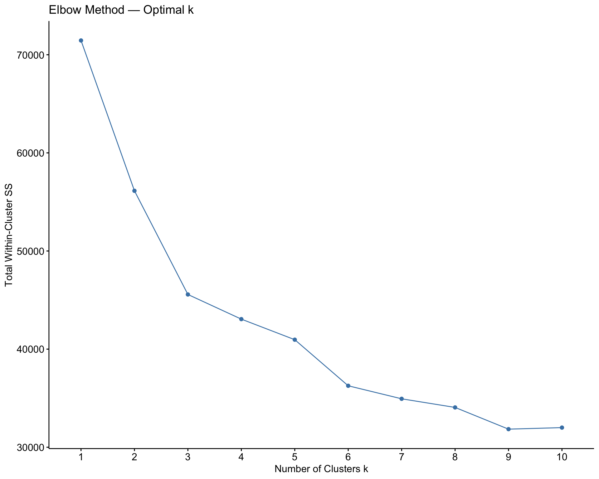
Answer:
The total within-cluster sum of squares decreases as \(k\) increases. This always happens because adding more clusters gives the model more flexibility. Therefore, we should not simply choose the value of \(k\) with the smallest total within-cluster sum of squares. Instead, we look for an elbow where the improvement begins to slow down. In this wine example, \(k = 2\) is easy to interpret because it appears to capture a major red-versus-white distinction, although other values of \(k\) may reveal more detailed subgroups.
Question 8. Principal Component Analysis
princ_wine <- prcomp(wine_scaled, scale. = FALSE)

fviz_eig(princ_wine, addlabels = TRUE, ncp = 10,
main = "Wine PCs") 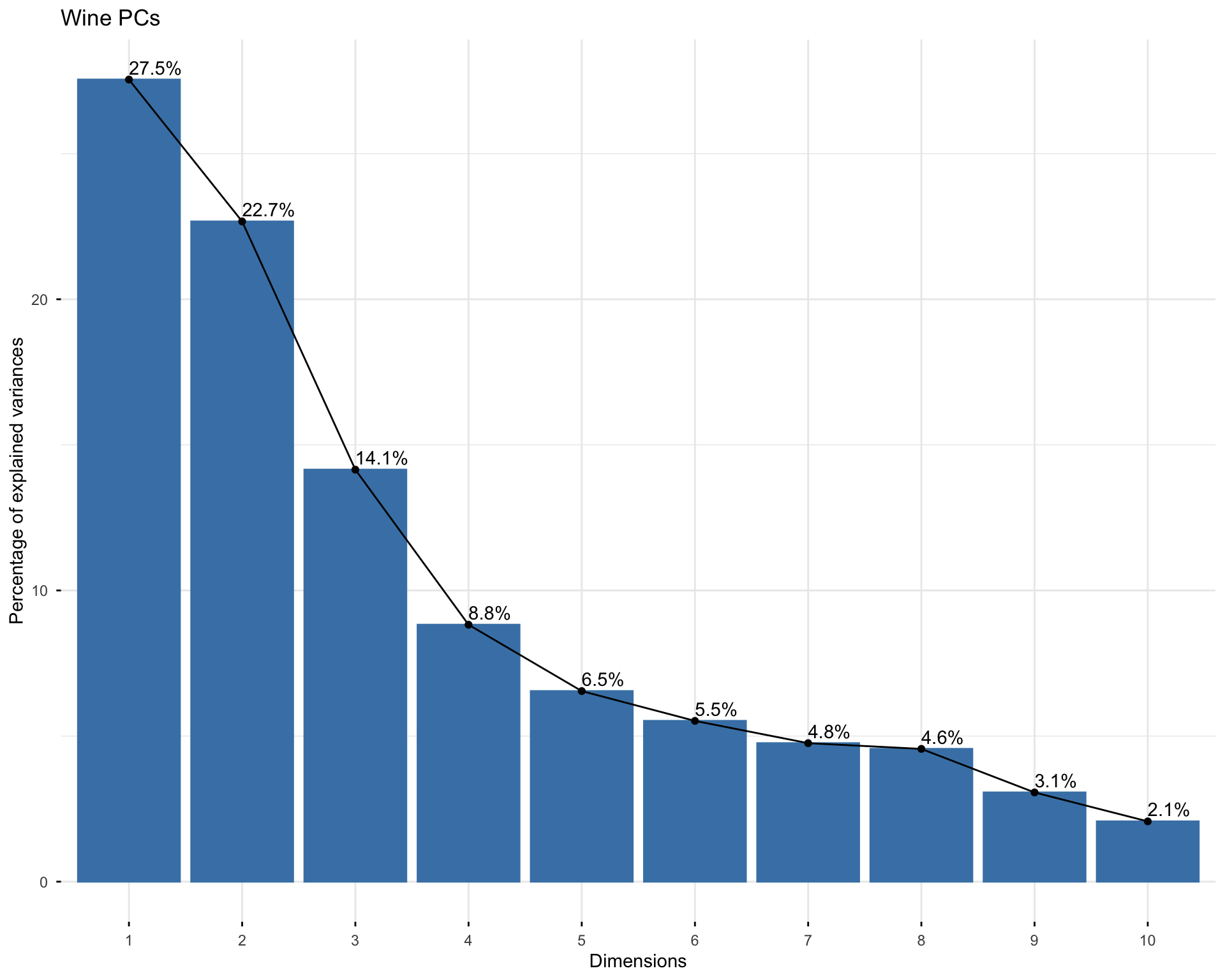
summary(princ_wine)$importance[, 1:5] PC1 PC2 PC3 PC4 PC5
Standard deviation 1.740652 1.579185 1.247536 0.985166 0.8484544
Proportion of Variance 0.275440 0.226710 0.141490 0.088230 0.0654400
Cumulative Proportion 0.275440 0.502150 0.643640 0.731870 0.7973200pca_importance <- summary(princ_wine)$importance
pca_importance["Proportion of Variance", 1:2] PC1 PC2
0.27544 0.22671 sum(pca_importance["Proportion of Variance", 1:2])[1] 0.50215Answer:
The first two principal components explain the share of variation shown in the PCA summary table. The scree plot shows how quickly the explained variation drops as we move from PC1 to later components. If the first few bars are much larger than the later bars, then the first few principal components capture a substantial amount of information. In this data set, the first two principal components are useful for visualization, but they do not contain all of the information in the original chemical variables.
Question 9. Interpret the loading matrix
t(round(princ_wine$rotation, 1))[1:2, ] acidity_fixed acidity_volatile acidity_citric residual_sugar chlorides
PC1 -0.2 -0.4 0.2 0.3 -0.3
PC2 -0.3 -0.1 -0.2 -0.3 -0.3
so2_free so2_tot density pH so4_2 alcohol
PC1 0.4 0.5 0.0 -0.2 -0.3 -0.1
PC2 -0.1 -0.1 -0.6 0.2 -0.2 0.5loadings_df <- princ_wine$rotation |>
as.data.frame() |>
rownames_to_column("variable") |>
select(variable, PC1, PC2) |>
mutate(
abs_PC1 = abs(PC1),
abs_PC2 = abs(PC2)
)
loadings_df |>
arrange(desc(abs_PC1)) |>
select(variable, PC1) |>
head(5) variable PC1
1 so2_tot 0.4874181
2 so2_free 0.4309140
3 acidity_volatile -0.3807575
4 residual_sugar 0.3459199
5 so4_2 -0.2941352loadings_df |>
arrange(desc(abs_PC2)) |>
select(variable, PC2) |>
head(5) variable PC2
1 density -0.5840373
2 alcohol 0.4650577
3 acidity_fixed -0.3363545
4 residual_sugar -0.3299142
5 chlorides -0.3152580Answer:
The loading matrix shows that PC1 is mainly driven by sulfur dioxide and acidity-related variables. The largest PC1 loadings are for so2_tot, so2_free, acidity_volatile, residual_sugar, and so4_2. Because so2_tot and so2_free have large positive loadings, wines with higher PC1 values tend to have higher sulfur dioxide levels. Since acidity_volatile and so4_2 have negative loadings, wines with higher PC1 values tend to have lower volatile acidity and lower sulfate values.
PC2 is mainly driven by density, alcohol, fixed acidity, residual sugar, and chlorides. The largest PC2 loading is negative for density, while alcohol has a large positive loading. Therefore, wines with higher PC2 values tend to have higher alcohol and lower density. Since residual_sugar, acidity_fixed, and chlorides have negative loadings, higher PC2 values are also associated with lower sugar, lower fixed acidity, and lower chloride levels.
Overall, PC1 appears to separate wines based on sulfur dioxide and acidity composition, while PC2 appears to separate wines based on alcohol-density balance and related chemical characteristics.
Question 10. PCA scatter plot
Z <- predict(princ_wine, wine_scaled)

zpilot_df <- as.data.frame(Z[, 1:2]) |>
  mutate(Color  = wine$color,
         Quality = wine$quality)

ggplot(zpilot_df, aes(x = PC1, y = PC2, color = Color, size = Quality)) +
  geom_point(alpha = 0.1) +
  scale_size_continuous(range = c(3, 9), name = "Wine Quality") +
  labs(
    title = "Wine in PC Space",
    x = "Principal Component 1",
    y = "Principal Component 2",
    color = "Wine Color"
  ) +
  guides(
    color = guide_legend(override.aes = list(alpha = 1, size = 4)),
    size = guide_legend(override.aes = list(alpha = 1))
  )
Answer:
The PCA plot suggests that red and white wines differ in multivariate chemical composition. The two colors tend to occupy different regions of the PC1-PC2 space, although there may still be some overlap. This supports the earlier k-means result: even without using the color label, the chemical variables contain structure that helps separate red and white wines.
Discussion
Welcome to our Classwork 10 Discussion Board! 👋
This space is designed for you to engage with your classmates about the material covered in Classwork 10.
Whether you are looking to delve deeper into the content, share insights, or have questions about the content, this is the perfect place for you.
If you have any specific questions for Byeong-Hak (@bcdanl) regarding the Classwork 10 materials or need clarification on any points, don’t hesitate to ask here.
All comments will be stored here.
Let’s collaborate and learn from each other!