Association Rules

Music Data

Author

Byeong-Hak Choe

Published

April 29, 2026

Modified

May 3, 2026

📌 Overview

This classwork analyzes a music-listening transaction dataset using association rules.
Each transaction represents one listener, and each item represents one artist listened to by that listener.

We will use arules for transaction objects and association-rule mining.

library(tidyverse)
library(rmarkdown)
library(arules)
library(arulesViz)
library(plotly)

🎧 Load the Music Transaction Data

path_music <- "https://bcdanl.github.io/data/music_old.tsv"

music_eg <- read.transactions(
  file = path_music,
  format = "single",
  header = TRUE,
  cols = c(1, 2),
  rm.duplicates = TRUE
)

1️⃣ Column and Row Labels

Question 1

What do the labels for the column and the row of music_eg represent?

Answer

In the transaction matrix:

The columns represent artists.
The rows represent listeners.
A cell is marked as present when a listener listened to a given artist.

# First 10 artist labels
colnames(music_eg)[1:10]

 [1] "...and you will know us by the trail of dead"
 [2] "[unknown]"                                   
 [3] "2pac"                                        
 [4] "3 doors down"                                
 [5] "30 seconds to mars"                          
 [6] "311"                                         
 [7] "36 crazyfists"                               
 [8] "44"                                          
 [9] "50 cent"                                     
[10] "65daysofstatic"

# First 10 listener labels
rownames(music_eg)[1:10]

 [1] "1"     "1000"  "10000" "10002" "10003" "10004" "10006" "10007" "10008"
[10] "10009"

# All item labels are artist names
itemLabels(music_eg) |> head(10)

 [1] "...and you will know us by the trail of dead"
 [2] "[unknown]"                                   
 [3] "2pac"                                        
 [4] "3 doors down"                                
 [5] "30 seconds to mars"                          
 [6] "311"                                         
 [7] "36 crazyfists"                               
 [8] "44"                                          
 [9] "50 cent"                                     
[10] "65daysofstatic"

The transaction dataset can also be summarized using summary().

summary(music_eg)

transactions as itemMatrix in sparse format with
 15000 rows (elements/itemsets/transactions) and
 1004 columns (items) and a density of 0.01925312 

most frequent items:
            radiohead           the beatles              coldplay 
                 2704                  2668                  2378 
red hot chili peppers                  muse               (Other) 
                 1786                  1711                278705 

element (itemset/transaction) length distribution:
sizes
  1   2   3   4   5   6   7   8   9  10  11  12  13  14  15  16  17  18  19  20 
185 222 280 302 359 385 472 461 491 501 504 482 472 471 480 476 456 455 444 455 
 21  22  23  24  25  26  27  28  29  30  31  32  33  34  35  36  37  38  39  40 
436 478 426 438 408 446 417 375 348 340 316 293 274 286 238 208 193 181 128 102 
 41  42  43  44  45  46  47  48  49  50  51  52  54  55  63  76 
 93  61  55  36  23  15   6  11   2   1   5   3   1   2   1   1 

   Min. 1st Qu.  Median    Mean 3rd Qu.    Max. 
   1.00   11.00   19.00   19.33   27.00   76.00 

includes extended item information - examples:
                                        labels
1 ...and you will know us by the trail of dead
2                                    [unknown]
3                                         2pac

includes extended transaction information - examples:
  transactionID
1             1
2          1000
3         10000

We can visualize the transaction matrix using image().

image(music_eg)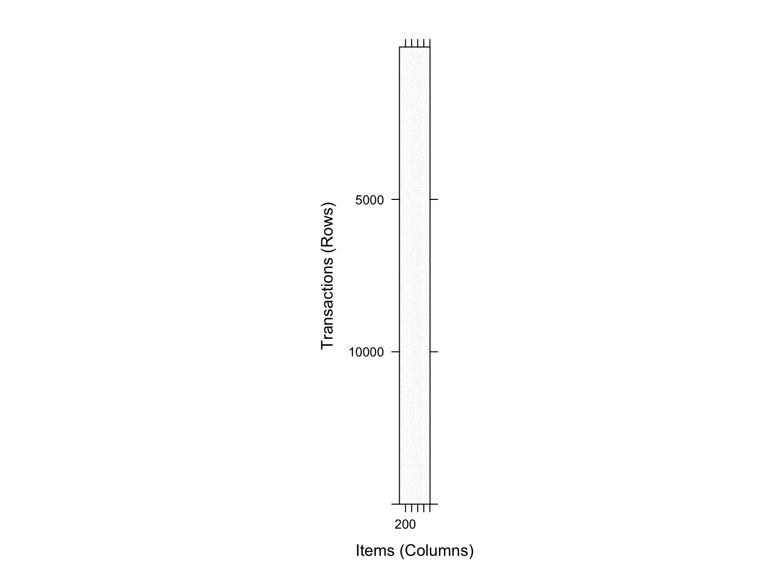

2️⃣ Transaction Sizes

Question 2a

What are the first quartile, the median, the third quartile, and the maximum of transaction sizes in music_eg?

Answer

A transaction size is the number of artists associated with one listener.

basket_sizes <- size(music_eg)

summary(basket_sizes)

   Min. 1st Qu.  Median    Mean 3rd Qu.    Max. 
   1.00   11.00   19.00   19.33   27.00   76.00

basket_size_summary <- tibble(transaction_size = basket_sizes) |>
  summarize(
    min = min(transaction_size),
    q1 = quantile(transaction_size, 0.25),
    median = median(transaction_size),
    mean = mean(transaction_size),
    q3 = quantile(transaction_size, 0.75),
    max = max(transaction_size)
  )

The values of interest are:

First quartile: 11
Median: 19
Third quartile: 27
Maximum: 76

Question 2b

Visualize the distribution of transaction sizes.

Answer

tibble(transaction_size = basket_sizes) |>
  ggplot(aes(x = transaction_size)) +
  geom_density(fill = "grey80", color = "black") +
  labs(
    title = "Distribution of Transaction Sizes",
    x = "Transaction Size: Number of Artists per Listener",
    y = "Density"
  ) +
  theme_minimal()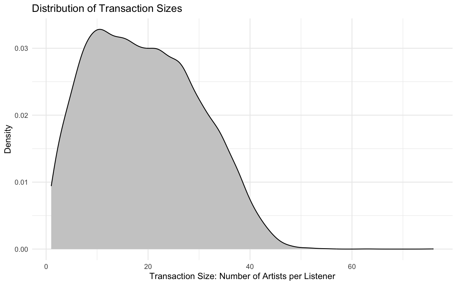

We can also use a histogram, which is often easier to interpret for count data.

tibble(transaction_size = basket_sizes) |>
  ggplot(aes(x = transaction_size)) +
  geom_histogram(binwidth = 5, fill = "grey80", color = "black") +
  labs(
    title = "Histogram of Transaction Sizes",
    x = "Transaction Size: Number of Artists per Listener",
    y = "Number of Listeners"
  ) +
  theme_minimal()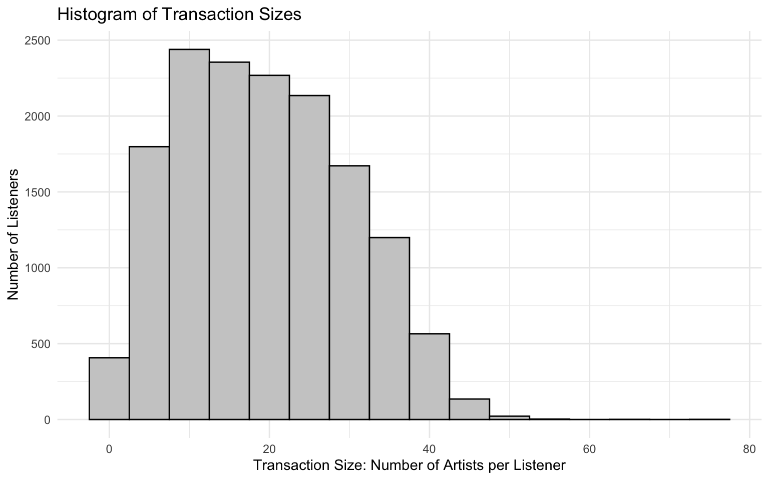

3️⃣ Item Frequencies

Question 3a

Find the top 50 most frequently occurring items in music_eg.
Also find the top 50 least frequently occurring items in music_eg.

Answer

First, we calculate the absolute frequency of each artist.

musicCount    <- itemFrequency(music_eg, "absolute")

musicCount_df <- data.frame(
  artist = names(musicCount),
  count = musicCount,
  row.names = NULL
)

musicCount_df |> 
  paged_table()

Top 50 Most Frequent Artists

top_50_artists <- musicCount_df |>
  slice_max(count, n = 50, with_ties = T) 

top_50_artists |> 
  paged_table()

Top 50 Least Frequent Artists

bottom_50_artists <- musicCount_df |>
  slice_min(count, n = 50, with_ties = T)

bottom_50_artists |> 
  paged_table()

Total Number of Artist Occurrences

musicCount_df |>
  summarize(total_artist_occurrences = sum(count))

  total_artist_occurrences
1                   289952

Visualization: Top 50 Most Frequent Artists

top_50_artists |>
  mutate(artist = fct_reorder(artist, count)) |>
  ggplot(aes(x = count, y = artist)) +
  geom_col(fill = "grey70", color = "black") +
  labs(
    title = "Top 50 Most Frequently Occurring Artists",
    x = "Number of Listeners",
    y = "Artist"
  ) +
  theme_minimal()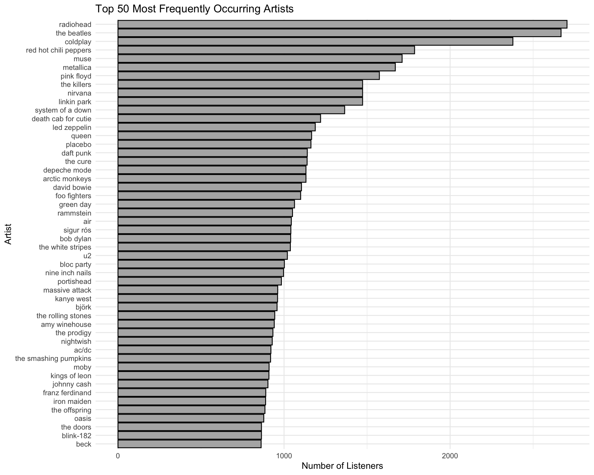

Visualization: Top 50 Least Frequent Artists

bottom_50_artists |>
  mutate(artist = fct_reorder(artist, -count)) |>
  ggplot(aes(x = count, y = artist)) +
  geom_col(fill = "grey70", color = "black") +
  labs(
    title = "Top 50 Least Frequently Occurring Artists",
    x = "Number of Listeners",
    y = "Artist"
  ) +
  theme_minimal()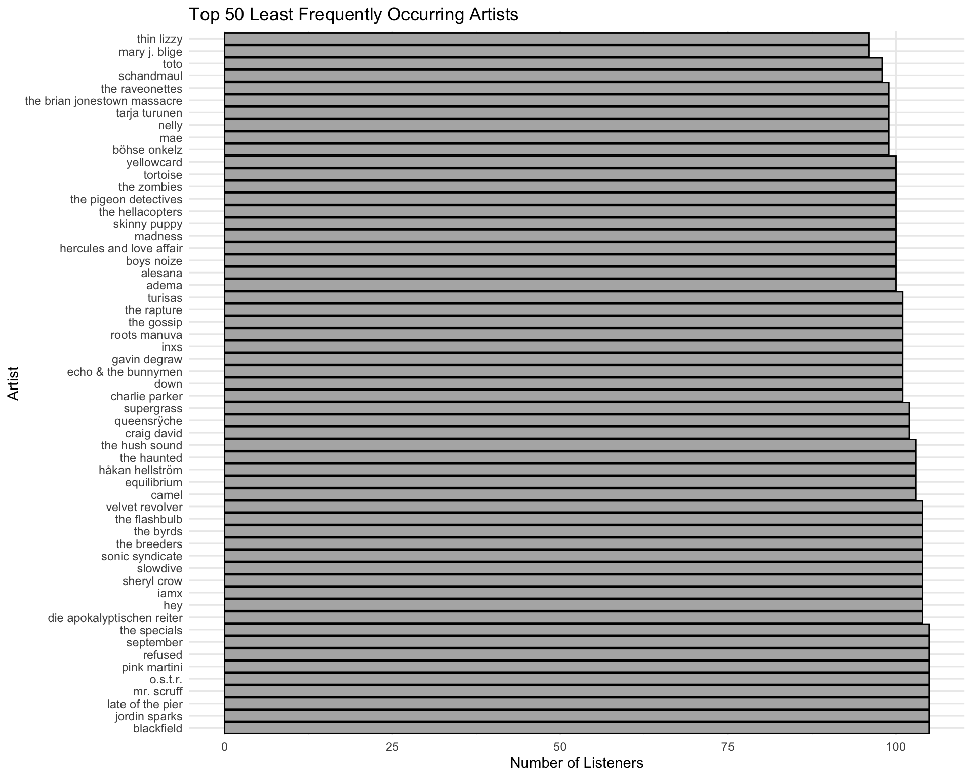

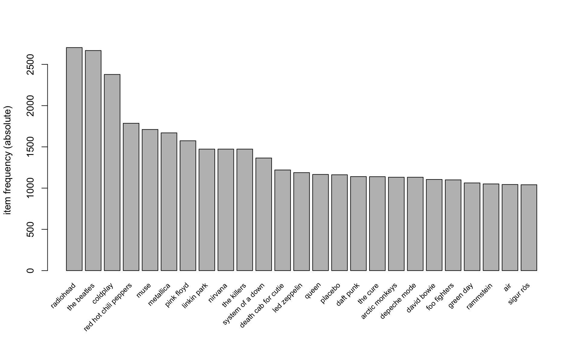
Question 3b [Bonus]

Visualize the distribution of item occurrence using itemFrequencyPlot().

Answer

The function itemFrequencyPlot() is a built-in function from the arules package.

itemFrequencyPlot(
  music_eg,
  type = "absolute",
  topN = 25,
  cex.names = 0.75
)

4️⃣ Association Rules

Before finding association rules, we subset the data to transactions with more than one artist.

musicbaskets_use <- music_eg[basket_sizes > 1]

musicbaskets_use

transactions in sparse format with
 14815 transactions (rows) and
 1004 items (columns)

Question 4a

From the subset of music_eg whose transaction size is greater than 1, find association rules with minimum support 0.01 and minimum confidence 0.5.

Answer

rules <- apriori(
  musicbaskets_use,
  parameter = list(
    support = 0.01,
    confidence = 0.5
  )
)

Apriori

Parameter specification:
 confidence minval smax arem  aval originalSupport maxtime support minlen
        0.5    0.1    1 none FALSE            TRUE       5    0.01      1
 maxlen target  ext
     10  rules TRUE

Algorithmic control:
 filter tree heap memopt load sort verbose
    0.1 TRUE TRUE  FALSE TRUE    2    TRUE

Absolute minimum support count: 148 

set item appearances ...[0 item(s)] done [0.00s].
set transactions ...[1004 item(s), 14815 transaction(s)] done [0.03s].
sorting and recoding items ... [658 item(s)] done [0.00s].
creating transaction tree ... done [0.00s].
checking subsets of size 1 2 3 4 done [0.01s].
writing ... [55 rule(s)] done [0.00s].
creating S4 object  ... done [0.00s].

summary(rules)

set of 55 rules

rule length distribution (lhs + rhs):sizes
 2  3 
16 39 

   Min. 1st Qu.  Median    Mean 3rd Qu.    Max. 
  2.000   2.000   3.000   2.709   3.000   3.000 

summary of quality measures:
    support          confidence        coverage            lift       
 Min.   :0.01006   Min.   :0.5006   Min.   :0.01606   Min.   : 2.747  
 1st Qu.:0.01060   1st Qu.:0.5219   1st Qu.:0.01839   1st Qu.: 3.065  
 Median :0.01154   Median :0.5498   Median :0.02140   Median : 3.238  
 Mean   :0.01321   Mean   :0.5553   Mean   :0.02410   Mean   : 3.877  
 3rd Qu.:0.01387   3rd Qu.:0.5839   3rd Qu.:0.02683   3rd Qu.: 3.688  
 Max.   :0.02997   Max.   :0.6627   Max.   :0.05987   Max.   :13.271  
     count      
 Min.   :149.0  
 1st Qu.:157.0  
 Median :171.0  
 Mean   :195.6  
 3rd Qu.:205.5  
 Max.   :444.0  

mining info:
             data ntransactions support confidence
 musicbaskets_use         14815    0.01        0.5
                                                                                 call
 apriori(data = musicbaskets_use, parameter = list(support = 0.01, confidence = 0.5))

Most rules have length 2 or 3:
- 16 rules are simple: {artist A} → {artist B}
- 39 rules are longer: {artist A, artist B} → {artist C}
Support: 1.01% to 3.00%
- Each rule appears in about 1% to 3% of all music baskets.
Confidence: 50.1% to 66.3%
- Among listeners with the artist(s) on the left-hand side, about half to two-thirds also have the artist on the right-hand side.
Lift: 2.75 to 13.27
- These rules show positive associations, meaning the artists appear together more often than expected by chance.
Count: 149 to 444
- Each rule is based on at least 149 baskets, so the patterns are supported by a meaningful number of observations.

Sort the rules by lift.

rules_lift <- rules |>
  sort(by = "lift", decreasing = TRUE) |>
  head(n = 5)

Instead of relying only on inspect(), we can convert the rules to a tidy table.

rules_tbl <- rules_lift |> 
  as("data.frame") |>
  separate(
    col = rules,
    into = c("lhs", "rhs"),
    sep = " => "
  )

rules_tbl |>
  arrange(-lift) |> 
  paged_table()

Scatter Plot of Rules

plot(rules_lift)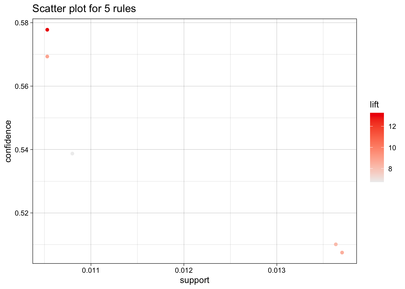

Graph Plot of Rules

plot(rules_lift, method = "graph")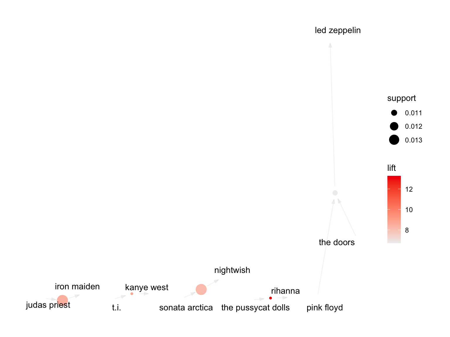

An interactive graph can also be created using the HTML widget engine.

plot(rules_lift, method = "graph", engine = "htmlwidget")

Question 4b

Pick one rule from Question 4a. Interpret the following qualities of the rule you pick:

support
confidence
coverage
lift
count

Answer

Here, we pick one rule from the rules generated in Question 4a. The following code selects one of the rules with high lift.

picked_rule <- rules_tbl |>
  arrange(desc(lift)) |>
  slice(1)

picked_rule |> 
  paged_table()

The selected rule is:

picked_lhs <- picked_rule$lhs
picked_rhs <- picked_rule$rhs

If a listener listened to {r picked_lhs}, then the listener is also likely to have listened to {r picked_rhs}.

The quality measures for this rule are:

picked_rule |>
  select(lhs, rhs, support, confidence, coverage, lift, count) |> 
  paged_table()

Interpretation

Let \(X\) be the item or itemset on the left-hand side, and let \(Y\) be the item on the right-hand side.

Support is the proportion of transactions that contain both \(X\) and \(Y\).
In this rule, support is 0.0105, which means about 1.05% of listeners have both the left-hand-side itemset and the right-hand-side item.
Confidence is the conditional probability of \(Y\) given \(X\).
In this rule, confidence is 0.5778, which means that among listeners who listened to {r picked_lhs}, about 57.78% also listened to {r picked_rhs}.
Coverage is the proportion of transactions that contain the left-hand-side itemset \(X\).
In this rule, coverage is 0.0182, which means about 1.82% of listeners listened to {r picked_lhs}.
Lift compares the observed confidence to the baseline probability of listening to the right-hand-side artist.
In this rule, lift is 13.271. Because this value is greater than 1, the left-hand-side itemset and the right-hand-side item occur together more often than expected under independence.
Count is the number of transactions that contain both \(X\) and \(Y\).
In this rule, count is 156, meaning that 156 listeners have both the left-hand-side itemset and the right-hand-side item.

Formula Summary

For a rule \(X \Rightarrow Y\):

\[ \text{support}(X \Rightarrow Y) = P(X \cap Y) \]

\[ \text{confidence}(X \Rightarrow Y) = P(Y \mid X) = \frac{P(X \cap Y)}{P(X)} \]

\[ \text{coverage}(X \Rightarrow Y) = P(X) \]

\[ \text{lift}(X \Rightarrow Y) = \frac{P(Y \mid X)}{P(Y)} \]

Lift can be interpreted as follows:

If lift is greater than 1, then \(X\) and \(Y\) appear together more often than expected.
If lift is close to 1, then \(X\) and \(Y\) appear together about as often as expected under independence.
If lift is less than 1, then \(X\) and \(Y\) appear together less often than expected.

Question 4c

Find at least 5 association rules for the item you pick by setting appropriate levels of minimum support and minimum confidence.

For this example, we will use coldplay as the right-hand-side item.

Answer

First, check whether coldplay is included in the transaction data.

any(itemLabels(music_eg) == "coldplay")

[1] TRUE

Now find association rules where the right-hand-side item is coldplay.

coldplay_rules <- apriori(
  musicbaskets_use,
  parameter = list(
    support = 0.005,
    confidence = 0.6
  ),
  appearance = list(
    rhs = "coldplay",
    default = "lhs"
  )
)

Apriori

Parameter specification:
 confidence minval smax arem  aval originalSupport maxtime support minlen
        0.6    0.1    1 none FALSE            TRUE       5   0.005      1
 maxlen target  ext
     10  rules TRUE

Algorithmic control:
 filter tree heap memopt load sort verbose
    0.1 TRUE TRUE  FALSE TRUE    2    TRUE

Absolute minimum support count: 74 

set item appearances ...[1 item(s)] done [0.00s].
set transactions ...[1004 item(s), 14815 transaction(s)] done [0.03s].
sorting and recoding items ... [1004 item(s)] done [0.00s].
creating transaction tree ... done [0.00s].
checking subsets of size 1 2 3 4 5 done [0.03s].
writing ... [41 rule(s)] done [0.00s].
creating S4 object  ... done [0.00s].

summary(coldplay_rules)

set of 41 rules

rule length distribution (lhs + rhs):sizes
 2  3  4 
 1 32  8 

   Min. 1st Qu.  Median    Mean 3rd Qu.    Max. 
  2.000   3.000   3.000   3.171   3.000   4.000 

summary of quality measures:
    support           confidence        coverage             lift      
 Min.   :0.005130   Min.   :0.6057   Min.   :0.006480   Min.   :3.773  
 1st Qu.:0.005400   1st Qu.:0.6270   1st Qu.:0.008100   1st Qu.:3.906  
 Median :0.005872   Median :0.6556   Median :0.009112   Median :4.085  
 Mean   :0.006982   Mean   :0.6665   Mean   :0.010587   Mean   :4.152  
 3rd Qu.:0.007695   3rd Qu.:0.6957   3rd Qu.:0.011070   3rd Qu.:4.334  
 Max.   :0.022545   Max.   :0.7917   Max.   :0.035370   Max.   :4.932  
     count      
 Min.   : 76.0  
 1st Qu.: 80.0  
 Median : 87.0  
 Mean   :103.4  
 3rd Qu.:114.0  
 Max.   :334.0  

mining info:
             data ntransactions support confidence
 musicbaskets_use         14815   0.005        0.6
                                                                                                                                        call
 apriori(data = musicbaskets_use, parameter = list(support = 0.005, confidence = 0.6), appearance = list(rhs = "coldplay", default = "lhs"))

Confidence: 60.6% to 79.2%
- Among listeners with the LHS artists, about 61% to 79% also include Coldplay.
Lift: 3.77 to 4.93
- These listeners are roughly 3.8 to 4.9 times more likely to include Coldplay than average.
Support: 0.51% to 2.25%
- These patterns appear in a small but meaningful share of all transactions.
Count: 76 to 334
- Each rule is supported by at least 76 transactions, indicating non-trivial sample size.

Sort the rules by lift.

coldplay_rules_lift <- coldplay_rules |>
  sort(by = "lift", decreasing = TRUE)

Convert the results into a tidy table.

coldplay_rules_tbl <- coldplay_rules_lift |> 
  as("data.frame") |>
  separate(
    col = rules,
    into = c("lhs", "rhs"),
    sep = " => "
  ) |>
  arrange(-lift)

coldplay_rules_tbl

                                           lhs        rhs     support
1                               {keane,travis} {coldplay} 0.005129936
2                                   {keane,u2} {coldplay} 0.005872427
3                          {keane,snow patrol} {coldplay} 0.007964900
4                                {keane,oasis} {coldplay} 0.006884914
5                               {oasis,travis} {coldplay} 0.005467432
6                       {arctic monkeys,keane} {coldplay} 0.005332433
7                {oasis,radiohead,the killers} {coldplay} 0.005197435
8                     {muse,oasis,the killers} {coldplay} 0.005264934
9                                {muse,travis} {coldplay} 0.005197435
10 {death cab for cutie,radiohead,the killers} {coldplay} 0.005467432
11                         {keane,the beatles} {coldplay} 0.006479919
12                 {death cab for cutie,oasis} {coldplay} 0.006007425
13                         {oasis,snow patrol} {coldplay} 0.007694904
14                                {keane,muse} {coldplay} 0.007762403
15                         {keane,the killers} {coldplay} 0.009652379
16                           {keane,radiohead} {coldplay} 0.007694904
17                          {bloc party,oasis} {coldplay} 0.005534931
18              {muse,the beatles,the killers} {coldplay} 0.005399933
19                         {oasis,the killers} {coldplay} 0.011272359
20                      {muse,oasis,radiohead} {coldplay} 0.005332433
21                          {radiohead,travis} {coldplay} 0.006682416
22                       {kaiser chiefs,oasis} {coldplay} 0.005264934
23                            {snow patrol,u2} {coldplay} 0.005872427
24         {red hot chili peppers,snow patrol} {coldplay} 0.006884914
25                                     {keane} {coldplay} 0.022544718
26               {bloc party,muse,the killers} {coldplay} 0.005804927
27         {radiohead,the beatles,the killers} {coldplay} 0.005872427
28                     {radiohead,snow patrol} {coldplay} 0.010192373
29                     {franz ferdinand,oasis} {coldplay} 0.006749916
30                                {blur,oasis} {coldplay} 0.005467432
31                        {the killers,travis} {coldplay} 0.005332433
32                         {oasis,the strokes} {coldplay} 0.006074924
33            {the killers,the postal service} {coldplay} 0.005467432
34               {oasis,radiohead,the beatles} {coldplay} 0.005399933
35                {arctic monkeys,snow patrol} {coldplay} 0.005804927
36                     {snow patrol,the kooks} {coldplay} 0.005669929
37                            {the killers,u2} {coldplay} 0.009179885
38           {death cab for cutie,snow patrol} {coldplay} 0.007694904
39                      {arctic monkeys,oasis} {coldplay} 0.008437395
40                                {placebo,u2} {coldplay} 0.005197435
41                                {muse,oasis} {coldplay} 0.010057374
   confidence    coverage     lift count
1   0.7916667 0.006479919 4.932103    76
2   0.7767857 0.007559906 4.839395    87
3   0.7564103 0.010529868 4.712455   118
4   0.7555556 0.009112386 4.707130   102
5   0.7431193 0.007357408 4.629652    81
6   0.7247706 0.007357408 4.515339    79
7   0.7196262 0.007222410 4.483289    77
8   0.7155963 0.007357408 4.458183    78
9   0.7000000 0.007424907 4.361018    77
10  0.6982759 0.007829902 4.350276    81
11  0.6956522 0.009314884 4.333931    96
12  0.6953125 0.008639892 4.331814    89
13  0.6951220 0.011069862 4.330627   114
14  0.6886228 0.011272359 4.290137   115
15  0.6777251 0.014242322 4.222245   143
16  0.6666667 0.011542356 4.153350   114
17  0.6666667 0.008302396 4.153350    82
18  0.6666667 0.008099899 4.153350    80
19  0.6626984 0.017009787 4.128628   167
20  0.6583333 0.008099899 4.101433    79
21  0.6556291 0.010192373 4.084586    99
22  0.6500000 0.008099899 4.049516    78
23  0.6444444 0.009112386 4.014905    87
24  0.6415094 0.010732366 3.996620   102
25  0.6374046 0.035369558 3.971047   334
26  0.6370370 0.009112386 3.968757    86
27  0.6350365 0.009247384 3.956293    87
28  0.6344538 0.016064799 3.952663   151
29  0.6329114 0.010664867 3.943054   100
30  0.6328125 0.008639892 3.942438    81
31  0.6269841 0.008504894 3.906127    79
32  0.6250000 0.009719879 3.893766    90
33  0.6230769 0.008774890 3.881785    81
34  0.6201550 0.008707391 3.863582    80
35  0.6187050 0.009382383 3.854548    86
36  0.6131387 0.009247384 3.819869    84
37  0.6126126 0.014984813 3.816592   136
38  0.6096257 0.012622342 3.797983   114
39  0.6067961 0.013904826 3.780355   125
40  0.6062992 0.008572393 3.777259    77
41  0.6056911 0.016604792 3.773471   149

The following table shows at least five rules for coldplay.

coldplay_rules_tbl |>
  slice_head(n = 5)

                  lhs        rhs     support confidence    coverage     lift
1      {keane,travis} {coldplay} 0.005129936  0.7916667 0.006479919 4.932103
2          {keane,u2} {coldplay} 0.005872427  0.7767857 0.007559906 4.839395
3 {keane,snow patrol} {coldplay} 0.007964900  0.7564103 0.010529868 4.712455
4       {keane,oasis} {coldplay} 0.006884914  0.7555556 0.009112386 4.707130
5      {oasis,travis} {coldplay} 0.005467432  0.7431193 0.007357408 4.629652
  count
1    76
2    87
3   118
4   102
5    81

Visualization of `coldplay` Rules

plot(coldplay_rules_lift)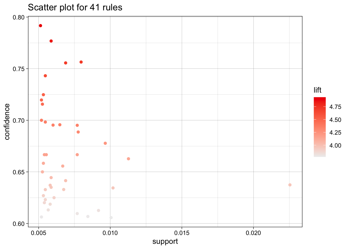

plot(coldplay_rules_lift, method = "graph")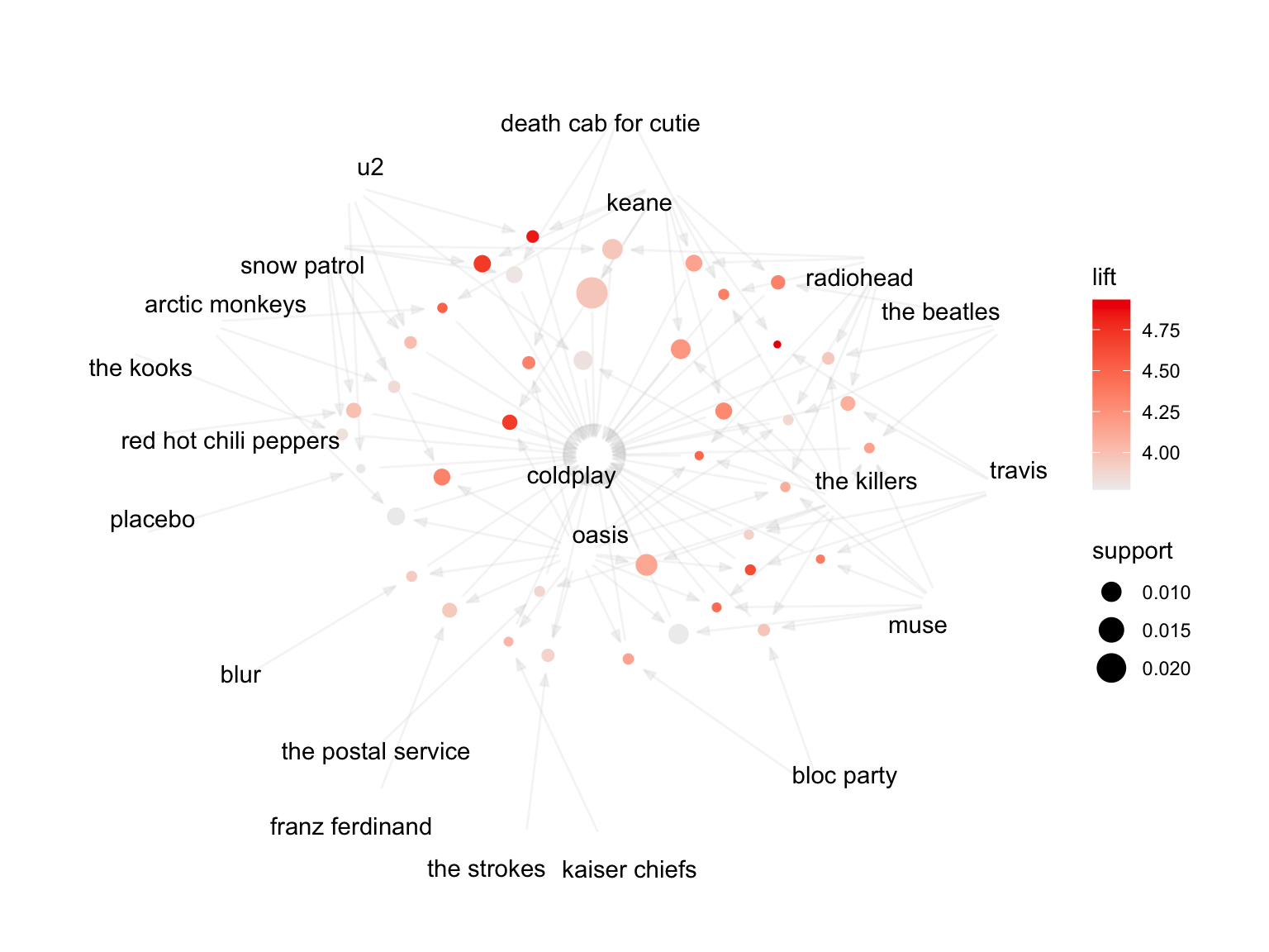

An interactive plot can also be created with plotly.

plot(coldplay_rules_lift, engine = "plotly")

✅ Conclusion

This homework used association-rule mining to identify relationships among artists in a music-listening dataset. The key steps were:

reading music listening data as transaction data;
summarizing transaction sizes;
identifying frequent and rare artists;
mining association rules using apriori();
interpreting support, confidence, coverage, lift, and count;
finding artist-specific rules for coldplay.

📌 Overview

🎧 Load the Music Transaction Data

1️⃣ Column and Row Labels

Question 1

Answer

2️⃣ Transaction Sizes

Question 2a

Answer

Question 2b

Answer

3️⃣ Item Frequencies

Question 3a

Answer

Top 50 Most Frequent Artists

Top 50 Least Frequent Artists

Total Number of Artist Occurrences

Visualization: Top 50 Most Frequent Artists

Visualization: Top 50 Least Frequent Artists

Question 3b [Bonus]

Answer

4️⃣ Association Rules

Question 4a

Answer

Scatter Plot of Rules

Graph Plot of Rules

Question 4b

Answer

Interpretation

Formula Summary

Question 4c

Answer

Visualization of coldplay Rules

✅ Conclusion

Visualization of `coldplay` Rules