library(tidyverse)
library(rmarkdown)

library(arules)
library(arulesViz)
library(plotly)Homework 6
Association Rules with Grocery Data
Direction
Please submit one Quarto Document of Homework 6 to Brightspace using the following file naming convention:
Example:
danl-320-hw6-choe-byeonghak.qmd
Due: May 6, 2026, 11:59 P.M. (ET)
Please send Byeong-Hak an email (
bchoe@geneseo.edu) if you have any questions.
Setup
📥 Load the Grocery Transaction Data
The data are stored in a single transaction format, where each row represents one item purchased in one transaction.
grocery <- read.transactions(
  "https://bcdanl.github.io/data/market_basket.tsv",
  format = "single",
  header = TRUE,
  cols = c(1, 2),
  rm.duplicates = TRUE
)
Question 1. 🏷️ Transaction and Item Labels
What do the labels for the column and the row of grocery represent?
Show answer
In the transaction matrix:
- The columns represent grocery item categories.
- The rows represent individual grocery transactions.
colnames(grocery)[1:10] [1] "abrasive cleaner" "artif. sweetener" "baby cosmetics" "baby food"
[5] "bags" "baking powder" "bathroom cleaner" "beef"
[9] "berries" "beverages" rownames(grocery)[1:10] [1] "1" "10" "100" "1000" "1001" "1002" "1003" "1004" "1005" "1006"itemLabels(grocery)[1:20] [1] "abrasive cleaner" "artif. sweetener" "baby cosmetics" "baby food"
[5] "bags" "baking powder" "bathroom cleaner" "beef"
[9] "berries" "beverages" "bottled beer" "bottled water"
[13] "brandy" "brown bread" "butter" "butter milk"
[17] "cake bar" "candles" "candy" "canned beer" The first few column labels show item categories, such as grocery product names. The row labels identify individual transactions.
A transaction matrix is a sparse binary matrix. A value of TRUE or 1 means that a given item appeared in a given transaction, while a value of FALSE or 0 means that it did not.
summary(grocery)transactions as itemMatrix in sparse format with
9835 rows (elements/itemsets/transactions) and
169 columns (items) and a density of 0.02609085
most frequent items:
whole milk other vegetables rolls/buns soda
2513 1903 1809 1715
yogurt (Other)
1372 34054
element (itemset/transaction) length distribution:
sizes
1 2 3 4 5 6 7 8 9 10 11 12 13 14 15 16
2159 1643 1300 1004 855 645 545 438 350 246 182 117 78 77 55 46
17 18 19 20 21 22 23 24 26 27 28 29 32
29 14 14 9 11 4 6 1 1 1 1 3 1
Min. 1st Qu. Median Mean 3rd Qu. Max.
1.000 2.000 3.000 4.409 6.000 32.000
includes extended item information - examples:
labels
1 abrasive cleaner
2 artif. sweetener
3 baby cosmetics
includes extended transaction information - examples:
transactionID
1 1
2 10
3 100Question 2. 📦 Transaction Size Distribution
What are the first quartile, median, third quartile, and maximum of transaction sizes in grocery? Visualize the distribution of transaction sizes.
Show answer
The transaction size is the number of items purchased in each transaction.
basket_sizes <- size(grocery)

summary(basket_sizes)
Min. 1st Qu. Median Mean 3rd Qu. Max.
1.000 2.000 3.000 4.409 6.000 32.000 A tidy summary table is shown below.
transaction_size_summary <- tibble(
  statistic = c("Minimum", "First quartile", "Median", "Mean", "Third quartile", "Maximum"),
  value = as.numeric(summary(basket_sizes))
)

transaction_size_summary
# A tibble: 6 × 2
statistic value
<chr> <dbl>
1 Minimum 1
2 First quartile 2
3 Median 3
4 Mean 4.41
5 Third quartile 6
6 Maximum 32 📊 Density Plot of Transaction Sizes
basket_sizes_df <- tibble(
  transaction_id = rownames(grocery),
  transaction_size = basket_sizes
)

basket_sizes_df |>
  ggplot(aes(x = transaction_size)) +
  geom_density(fill = "gray80", color = "black") +
  labs(
    title = "Distribution of Grocery Transaction Sizes",
    x = "Number of items in transaction",
    y = "Density"
  ) +
  theme_minimal()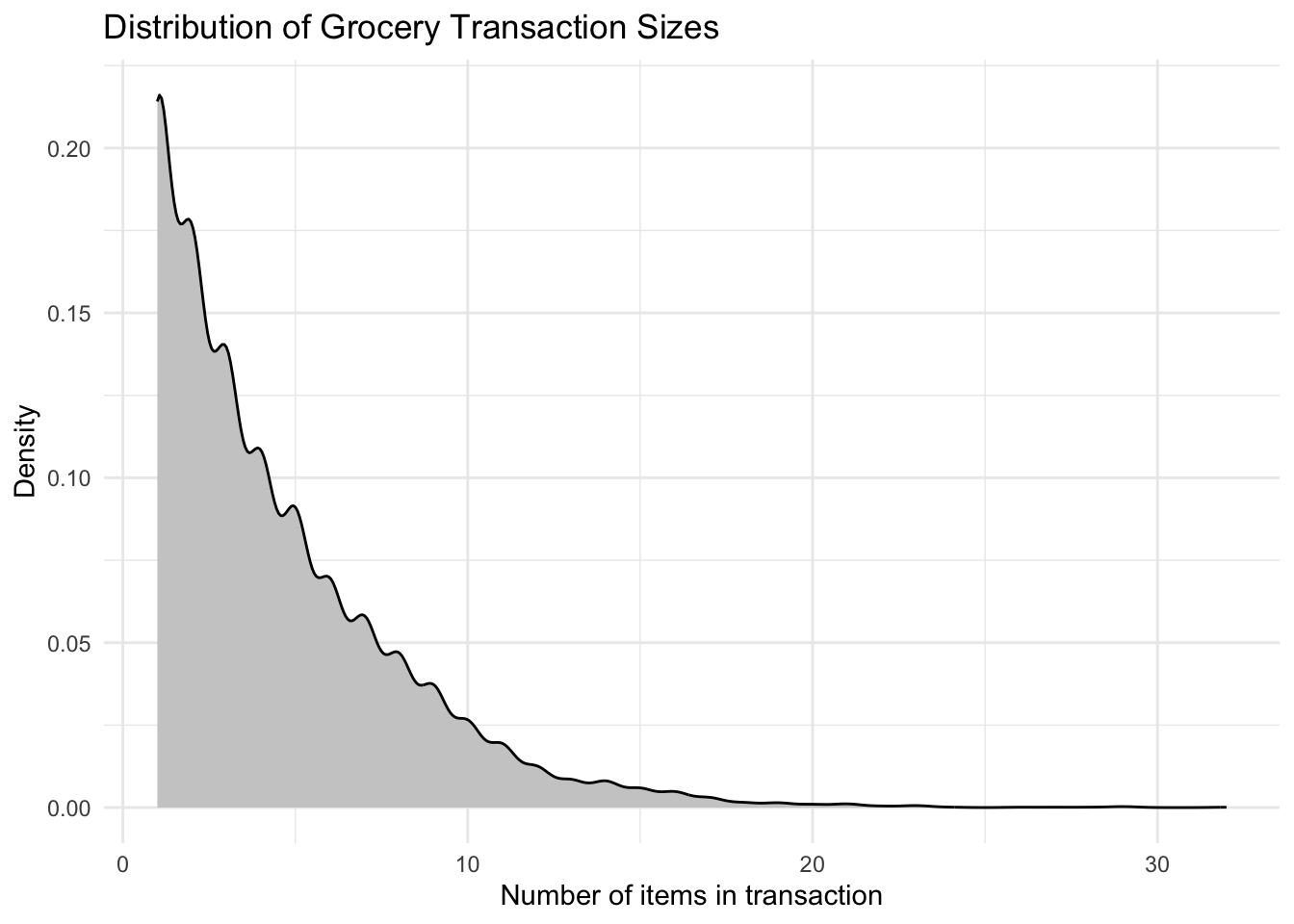
Most transactions contain a relatively small number of items, while a smaller number of transactions contain many items.
Question 3. 🔝 Top 50 Most Frequently Purchased Items
Find the top 50 most frequently occurring items in grocery. Also, visualize the distribution of top 50 item occurrences in grocery.
Show answer
We first calculate the absolute frequency of each item and convert the result into a tidy data frame.
grocery_count <- itemFrequency(grocery, type = "absolute")

grocery_count_df <- tibble(
  item = names(grocery_count),
  count = as.numeric(grocery_count)
) |>
  arrange(desc(count))

grocery_top50 <- grocery_count_df |>
  slice_head(n = 50)

grocery_top50
# A tibble: 50 × 2
item count
<chr> <dbl>
1 whole milk 2513
2 other vegetables 1903
3 rolls/buns 1809
4 soda 1715
5 yogurt 1372
6 bottled water 1087
7 root vegetables 1072
8 tropical fruit 1032
9 shopping bags 969
10 sausage 924
# ℹ 40 more rows📊 arules Frequency Plot
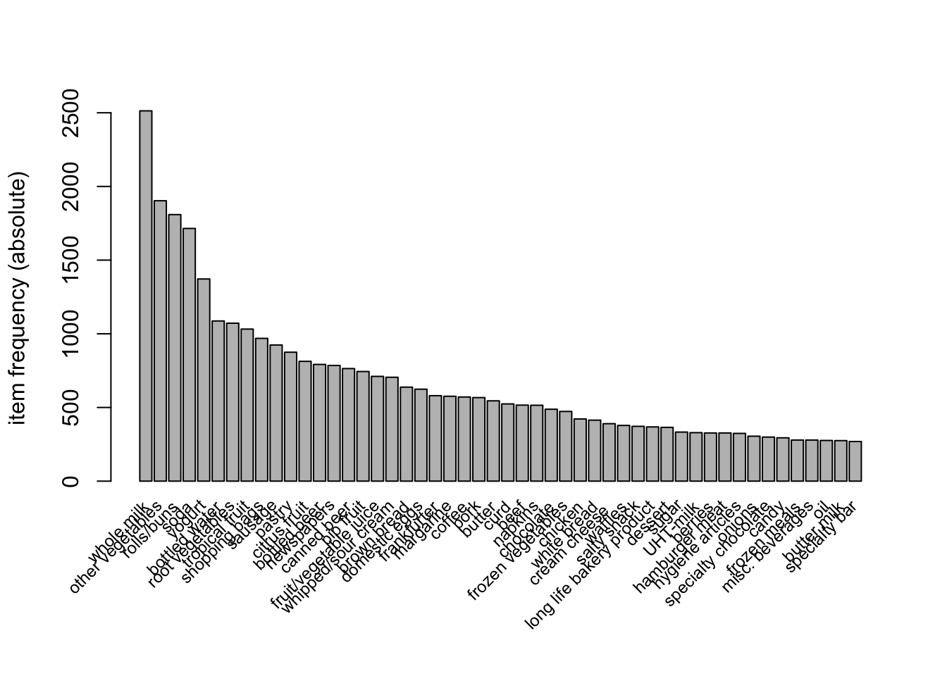
The itemFrequencyPlot() function gives a quick visualization directly from the transaction object.
itemFrequencyPlot(
  grocery,
  type = "absolute",
  topN = 50,
  cex.names = 0.75
)
📊 Alternative ggplot Bar Chart of Top 50 Items
grocery_top50 |>
  mutate(item = fct_reorder(item, count)) |>
  ggplot(aes(x = item, y = count)) +
  geom_col(color = "black", fill = "gray75") +
  coord_flip() +
  labs(
    title = "Top 50 Most Frequently Purchased Grocery Items",
    x = "Item",
    y = "Number of transactions"
  ) +
  theme_minimal()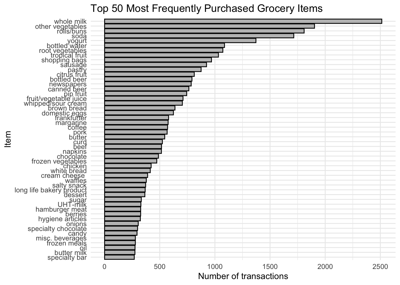
The most frequently purchased items are the items that appear in the largest number of transactions.
Question 4. ⛏️ Association Rules from Grocery Transactions
From the subset of grocery whose transaction size is greater than 1, find association rules with:
- minimum support =
0.01, - minimum confidence =
0.25, and - minimum rule length =
2.
Find the top 10 rules in terms of lift values.
Show answer
We first keep only transactions with more than one item because association rules require relationships across items.
grocery_use <- grocery[basket_sizes > 1]

summary(grocery_use)
transactions as itemMatrix in sparse format with
7676 rows (elements/itemsets/transactions) and
169 columns (items) and a density of 0.03176503
most frequent items:
whole milk other vegetables rolls/buns soda
2392 1841 1700 1559
yogurt (Other)
1332 32383
element (itemset/transaction) length distribution:
sizes
2 3 4 5 6 7 8 9 10 11 12 13 14 15 16 17
1643 1300 1004 855 645 545 438 350 246 182 117 78 77 55 46 29
18 19 20 21 22 23 24 26 27 28 29 32
14 14 9 11 4 6 1 1 1 1 3 1
Min. 1st Qu. Median Mean 3rd Qu. Max.
2.000 3.000 4.000 5.368 7.000 32.000
includes extended item information - examples:
labels
1 abrasive cleaner
2 artif. sweetener
3 baby cosmetics
includes extended transaction information - examples:
transactionID
1 1
2 10
3 100Now we run the Apriori algorithm.
rules <- apriori(
  grocery_use,
  parameter = list(
    support = 0.01,
    confidence = 0.25,
    minlen = 2
  )
)
Apriori
Parameter specification:
confidence minval smax arem aval originalSupport maxtime support minlen
0.25 0.1 1 none FALSE TRUE 5 0.01 2
maxlen target ext
10 rules TRUE
Algorithmic control:
filter tree heap memopt load sort verbose
0.1 TRUE TRUE FALSE TRUE 2 TRUE
Absolute minimum support count: 76
set item appearances ...[0 item(s)] done [0.00s].
set transactions ...[169 item(s), 7676 transaction(s)] done [0.00s].
sorting and recoding items ... [98 item(s)] done [0.00s].
creating transaction tree ... done [0.00s].
checking subsets of size 1 2 3 4 done [0.00s].
writing ... [310 rule(s)] done [0.00s].
creating S4 object ... done [0.00s].summary(rules)set of 310 rules
rule length distribution (lhs + rhs):sizes
2 3 4
134 172 4
Min. 1st Qu. Median Mean 3rd Qu. Max.
2.000 2.000 3.000 2.581 3.000 4.000
summary of quality measures:
support confidence coverage lift
Min. :0.01003 Min. :0.2508 Min. :0.01655 Min. :0.811
1st Qu.:0.01159 1st Qu.:0.2973 1st Qu.:0.03114 1st Qu.:1.323
Median :0.01381 Median :0.3577 Median :0.04123 Median :1.542
Mean :0.01858 Mean :0.3740 Mean :0.05294 Mean :1.612
3rd Qu.:0.02084 3rd Qu.:0.4371 3rd Qu.:0.06217 3rd Qu.:1.856
Max. :0.09588 Max. :0.6389 Max. :0.31162 Max. :3.174
count
Min. : 77.0
1st Qu.: 89.0
Median :106.0
Mean :142.6
3rd Qu.:160.0
Max. :736.0
mining info:
data ntransactions support confidence
grocery_use 7676 0.01 0.25
call
apriori(data = grocery_use, parameter = list(support = 0.01, confidence = 0.25, minlen = 2))📋 Tidy Rule Table
The as("data.frame") function converts the rules into a data frame, which makes it easier to use tidyverse tools.
rules_lift <- rules |>
  sort(by = "lift", decreasing = TRUE) |>
  head(n = 5)

rules_df <- rules_lift |>
  as("data.frame") |>
  separate(
    col = rules,
    into = c("lhs", "rhs"),
    sep = " => "
  ) |>
  arrange(-lift)

rules_df
lhs rhs support confidence
1 {berries} {whipped/sour cream} 0.01159458 0.2807571
2 {beef,other vegetables} {root vegetables} 0.01016154 0.4020619
3 {other vegetables,tropical fruit} {pip fruit} 0.01211569 0.2634561
4 {beef,whole milk} {root vegetables} 0.01029182 0.3779904
5 {other vegetables,pip fruit} {tropical fruit} 0.01211569 0.3618677
coverage lift count
1 0.04129755 3.173920 89
2 0.02527358 2.947686 78
3 0.04598749 2.824426 93
4 0.02722772 2.771208 79
5 0.03348098 2.752920 93🔝 Top 10 Rules by Lift
top10_lift_rules <- rules_df |>
  slice_max(lift, n = 10)

top10_lift_rules
lhs rhs support confidence
1 {berries} {whipped/sour cream} 0.01159458 0.2807571
2 {beef,other vegetables} {root vegetables} 0.01016154 0.4020619
3 {other vegetables,tropical fruit} {pip fruit} 0.01211569 0.2634561
4 {beef,whole milk} {root vegetables} 0.01029182 0.3779904
5 {other vegetables,pip fruit} {tropical fruit} 0.01211569 0.3618677
coverage lift count
1 0.04129755 3.173920 89
2 0.02527358 2.947686 78
3 0.04598749 2.824426 93
4 0.02722772 2.771208 79
5 0.03348098 2.752920 93The top rules by lift identify item combinations that occur together much more often than expected under independence.
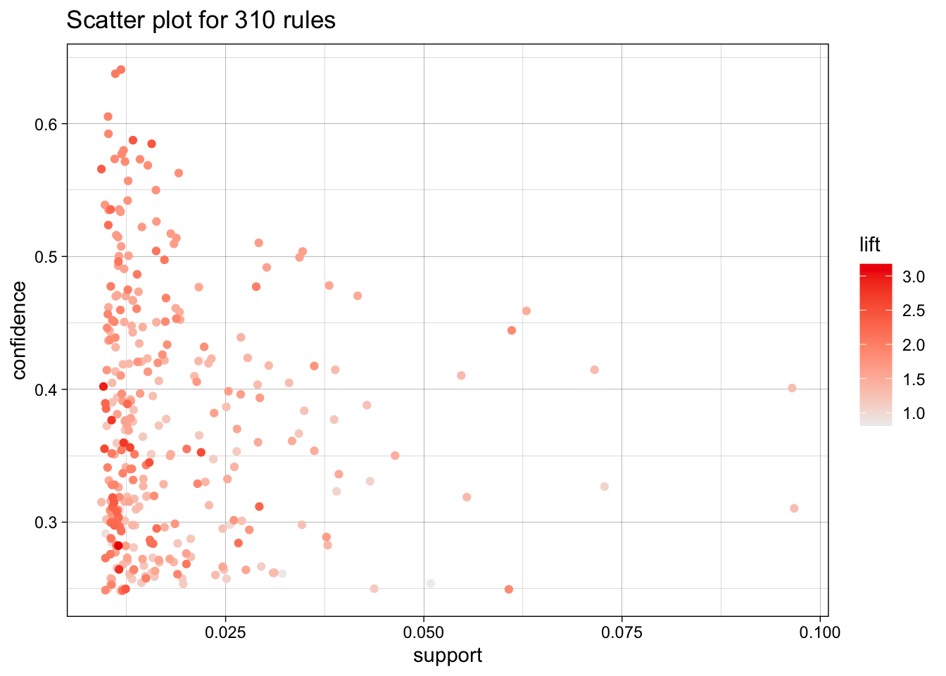
📈 Rule Plot
plot(
  rules,
  measure = c("support", "confidence"),
  shading = "lift",
  interactive = FALSE
)
🕸️ Rule Graph
pinterac <- plot(rules, method = "graph", engine = "htmlwidget")The graph plot is useful for exploring relationships among items, but it can be visually crowded when there are many rules.
🔝 Top 10 Rules by Confidence
top10_confidence_rules <- rules_df |>
  slice_max(confidence, n = 10)

top10_confidence_rules
lhs rhs support confidence
1 {beef,other vegetables} {root vegetables} 0.01016154 0.4020619
2 {beef,whole milk} {root vegetables} 0.01029182 0.3779904
3 {other vegetables,pip fruit} {tropical fruit} 0.01211569 0.3618677
4 {berries} {whipped/sour cream} 0.01159458 0.2807571
5 {other vegetables,tropical fruit} {pip fruit} 0.01211569 0.2634561
coverage lift count
1 0.02527358 2.947686 78
2 0.02722772 2.771208 79
3 0.03348098 2.752920 93
4 0.04129755 3.173920 89
5 0.04598749 2.824426 93Question 5. 🧠 Interpret the Rule with the Highest Lift
Interpret the following qualities of the rule with the highest lift:
- confidence,
- coverage, and
- lift.
Show answer
We identify the rule with the highest lift.
highest_lift_rule <- rules_df |>
  slice_max(lift, n = 1)

highest_lift_rule
lhs rhs support confidence coverage lift count
1 {berries} {whipped/sour cream} 0.01159458 0.2807571 0.04129755 3.17392 89Let the rule be written as:
\[ X \Rightarrow Y \]
where \(X\) is the item or set of items on the left-hand side and \(Y\) is the item or set of items on the right-hand side.
Interpretation
The rule found here is:
{berries} => {whipped/sour cream}This means that customers who bought berries were also likely to buy whipped/sour cream.
Confidence = 0.2808 means that among customers who bought berries, about 28.1% also bought whipped/sour cream.
Coverage = 0.0413 means that about 4.1% of transactions contained berries. In other words, berries were not extremely common, but they appeared often enough to generate a meaningful rule.
Lift = 3.1739 means that customers who bought berries were about 3.17 times more likely to buy whipped/sour cream than an average customer. Because the lift is greater than 1, berries and whipped/sour cream are purchased together more often than we would expect by chance.
Overall, this rule suggests a strong positive association between berries and whipped/sour cream. This makes intuitive sense because customers may buy berries and whipped or sour cream together for desserts, toppings, or fruit-based snacks.
Question 6. 🥛 What Did Customers Buy Before Buying Whole Milk?
What item(s) did customers buy before buying whole milk?
For this milk rule, use:
- minimum support =
0.01, - minimum confidence =
0.25, and - minimum rule length =
2.
Show answer
To answer this question, we place whole milk on the right-hand side of the rule. This means we are looking for rules of the form:
\[ X \Rightarrow \{\text{whole milk}\} \]
milk_rules_rhs <- apriori(
  grocery_use,
  parameter = list(
    support = 0.01,
    confidence = 0.25,
    minlen = 2
  ),
  appearance = list(
    default = "lhs",
    rhs = "whole milk"
  )
)
Apriori
Parameter specification:
confidence minval smax arem aval originalSupport maxtime support minlen
0.25 0.1 1 none FALSE TRUE 5 0.01 2
maxlen target ext
10 rules TRUE
Algorithmic control:
filter tree heap memopt load sort verbose
0.1 TRUE TRUE FALSE TRUE 2 TRUE
Absolute minimum support count: 76
set item appearances ...[1 item(s)] done [0.00s].
set transactions ...[169 item(s), 7676 transaction(s)] done [0.00s].
sorting and recoding items ... [98 item(s)] done [0.00s].
creating transaction tree ... done [0.00s].
checking subsets of size 1 2 3 4 done [0.00s].
writing ... [110 rule(s)] done [0.00s].
creating S4 object ... done [0.00s].summary(milk_rules_rhs)set of 110 rules
rule length distribution (lhs + rhs):sizes
2 3 4
53 56 1
Min. 1st Qu. Median Mean 3rd Qu. Max.
2.000 2.000 3.000 2.527 3.000 4.000
summary of quality measures:
support confidence coverage lift
Min. :0.01003 Min. :0.2527 Min. :0.01655 Min. :0.811
1st Qu.:0.01186 1st Qu.:0.3905 1st Qu.:0.02534 1st Qu.:1.253
Median :0.01472 Median :0.4371 Median :0.03439 Median :1.403
Mean :0.02086 Mean :0.4452 Mean :0.05055 Mean :1.429
3rd Qu.:0.02495 3rd Qu.:0.5041 3rd Qu.:0.05970 3rd Qu.:1.618
Max. :0.09588 Max. :0.6389 Max. :0.23984 Max. :2.050
count
Min. : 77.0
1st Qu.: 91.0
Median :113.0
Mean :160.1
3rd Qu.:191.5
Max. :736.0
mining info:
data ntransactions support confidence
grocery_use 7676 0.01 0.25
call
apriori(data = grocery_use, parameter = list(support = 0.01, confidence = 0.25, minlen = 2), appearance = list(default = "lhs", rhs = "whole milk"))milk_rules_rhs_df <- DATAFRAME(milk_rules_rhs, separate = TRUE) |>
as_tibble() |>
arrange(desc(lift))
milk_rules_rhs_df |>
paged_table()These rules show which items are associated with customers also buying whole milk.
Question 7. 🛍️ What Are Customers Who Bought Whole Milk Also Likely to Buy?
Find item(s) that customers who bought whole milk are also likely to buy.
Show answer
To answer this question, we place whole milk on the left-hand side of the rule. This means we are looking for rules of the form:
\[ \{\text{whole milk}\} \Rightarrow Y \]
milk_rules_lhs <- apriori(
  grocery_use,
  parameter = list(
    support = 0.01,
    confidence = 0.30,
    minlen = 2
  ),
  appearance = list(
    lhs = "whole milk",
    default = "rhs"
  )
)
Apriori
Parameter specification:
confidence minval smax arem aval originalSupport maxtime support minlen
0.3 0.1 1 none FALSE TRUE 5 0.01 2
maxlen target ext
10 rules TRUE
Algorithmic control:
filter tree heap memopt load sort verbose
0.1 TRUE TRUE FALSE TRUE 2 TRUE
Absolute minimum support count: 76
set item appearances ...[1 item(s)] done [0.00s].
set transactions ...[169 item(s), 7676 transaction(s)] done [0.00s].
sorting and recoding items ... [98 item(s)] done [0.00s].
creating transaction tree ... done [0.00s].
checking subsets of size 1 2 done [0.00s].
writing ... [1 rule(s)] done [0.00s].
creating S4 object ... done [0.00s].summary(milk_rules_lhs)set of 1 rules
rule length distribution (lhs + rhs):sizes
2
1
Min. 1st Qu. Median Mean 3rd Qu. Max.
2 2 2 2 2 2
summary of quality measures:
support confidence coverage lift
Min. :0.09588 Min. :0.3077 Min. :0.3116 Min. :1.283
1st Qu.:0.09588 1st Qu.:0.3077 1st Qu.:0.3116 1st Qu.:1.283
Median :0.09588 Median :0.3077 Median :0.3116 Median :1.283
Mean :0.09588 Mean :0.3077 Mean :0.3116 Mean :1.283
3rd Qu.:0.09588 3rd Qu.:0.3077 3rd Qu.:0.3116 3rd Qu.:1.283
Max. :0.09588 Max. :0.3077 Max. :0.3116 Max. :1.283
count
Min. :736
1st Qu.:736
Median :736
Mean :736
3rd Qu.:736
Max. :736
mining info:
data ntransactions support confidence
grocery_use 7676 0.01 0.3
call
apriori(data = grocery_use, parameter = list(support = 0.01, confidence = 0.3, minlen = 2), appearance = list(lhs = "whole milk", default = "rhs"))milk_rules_lhs_df <- DATAFRAME(milk_rules_lhs, separate = TRUE) |>
as_tibble() |>
arrange(desc(lift))
milk_rules_lhs_df# A tibble: 1 × 7
LHS RHS support confidence coverage lift count
<fct> <fct> <dbl> <dbl> <dbl> <dbl> <int>
1 {whole milk} {other vegetables} 0.0959 0.308 0.312 1.28 736The resulting rules describe items that are likely to appear in the same basket after whole milk appears on the left-hand side.
Question 8. 📉 Items Customers Are Less Likely to Buy Before Buying Whole Milk
Using the result of association rule mining in Question 4, find item(s) that customers are less likely to buy before buying whole milk. Why do you think those items are less likely to be purchased when customers buy whole milk?
Show answer
A rule with lift less than 1 indicates a negative association. In this context, the left-hand-side item and whole milk appear together less often than expected under independence.
We first filter the rules from Question 4 to rules where whole milk is on the right-hand side and the lift is less than 1.
less_likely_milk_rules <- rules_df |>
  filter(str_detect(rhs, "whole milk")) |>
  filter(lift < 1) |>
  arrange(lift)

less_likely_milk_rules
[1] lhs rhs support confidence coverage lift count
<0 rows> (or 0-length row.names)This table is empty. It means that within the rules generated using the Question 4 thresholds, there are no rules with whole milk on the right-hand side and lift less than 1.
We can also inspect the lowest-lift rules overall.
lowest_lift_rules <- rules_df |>
  arrange(lift) |>
  slice_head(n = 10)

lowest_lift_rules
lhs rhs support confidence
1 {other vegetables,pip fruit} {tropical fruit} 0.01211569 0.3618677
2 {beef,whole milk} {root vegetables} 0.01029182 0.3779904
3 {other vegetables,tropical fruit} {pip fruit} 0.01211569 0.2634561
4 {beef,other vegetables} {root vegetables} 0.01016154 0.4020619
5 {berries} {whipped/sour cream} 0.01159458 0.2807571
coverage lift count
1 0.03348098 2.752920 93
2 0.02722772 2.771208 79
3 0.04598749 2.824426 93
4 0.02527358 2.947686 78
5 0.04129755 3.173920 89Interpretation
Rules with lift less than 1 suggest that the items appear together less often than expected. For example, if a rule involving bottled beer and whole milk has lift below 1, it means customers who buy bottled beer are less likely than the average customer to also buy whole milk.
One possible explanation is that these products may belong to different shopping occasions. For example, customers buying beer may be shopping for entertainment, parties, or beverages, while customers buying whole milk may be shopping for regular household groceries, breakfast items, or cooking ingredients.
This does not mean that customers never buy the items together. It only means that the items occur together less often than expected based on their individual frequencies.