Homework 5

Hierarchical Clustering and PCA with Bloomberg COVID Resilience Rankings

Author

Byeong-Hak Choe

Published

April 20, 2026

Modified

May 4, 2026

Direction

Please submit one Quarto Document of Homework 5 to Brightspace using the following file naming convention:
Example:
- danl-320-hw5-choe-byeonghak.qmd
Due: April 27, 2026, 11:59 P.M. (ET)
Please send Byeong-Hak an email (bchoe@geneseo.edu) if you have any questions.

Setup

library(tidyverse)
library(rmarkdown)
library(hrbrthemes)
library(ggthemes)

library(ggrepel)
library(factoextra)
library(cluster)
library(fpc)


theme_set(theme_ipsum())

scale_colour_discrete <- function(...) scale_color_colorblind(...)
scale_fill_discrete <- function(...) scale_fill_colorblind(...)

url <- "http://bcdanl.github.io/data/bloomberg-covid-resilence-ranking.csv"
bloomberg <- read_csv(url)

paged_table(bloomberg)

Data Description

The dataset contains Bloomberg’s COVID resilience measures for a set of countries in November 2021 and December 2021.

Each row is a country-month observation.

Variable Descriptions

Variable	Description
`country`	Country or economy name
`year`	Year of observation
`month`	Month of observation (`11` for November, `12` for December)
`RANK`	Bloomberg resilience ranking
`CHANGE`	Change in ranking from the previous release
`BLOOMBERG RESILIENCE SCORE`	Overall Bloomberg resilience score
`PEOPLE COVERED BY VACCINES`	Share of people covered by vaccines
`LOCKDOWN SEVERITY`	Severity of lockdown restrictions
`FLIGHT CAPACITY`	Flight capacity measure
`VACCINATED TRAVEL ROUTES`	Measure of travel routes available to vaccinated travelers
`1-MONTH CASES PER 100,000`	COVID cases per 100,000 people over the past month
`3-MONTH CASE FATALITY RATE`	Case fatality rate over the past three months
`TOTAL DEATHS PER 1 MILLION`	Total COVID deaths per one million people
`POSITIVE TEST RATE`	Test positivity rate
`COMMUNITY MOBILITY`	Community mobility measure
`2021 GDP GROWTH FORECAST`	Forecasted GDP growth for 2021
`UNIVERSAL HEALTHCARE COVERAGE`	Universal healthcare coverage index
`HUMAN DEVELOPMENT INDEX`	Human Development Index
`VACCINE DOSES PER 100`	Vaccine doses administered per 100 people

Overview

In this homework, you will analyze the Bloomberg COVID Resilience Rankings data for November 2021 and December 2021.

You will perform the following for each month separately:

Data preparation
Hierarchical clustering with 5 clusters
Principal component analysis (PCA)
Interpretation of clustering and PCA results

Instructions

Do not use country, year, month, CHANGE, and BLOOMBERG RESILIENCE SCORE as analysis variables.
Because some variables contain missing values, replace missing values in numeric analysis variables with the variable mean within that month-specific dataset.

bloomberg <- bloomberg |> mutate_if(is.numeric, 
                        funs(
                          ifelse(is.na(.), 
                                 mean(., na.rm=T), .)
                             )
                        )

For hierarchical clustering, use:
- Euclidean distance
- Ward’s method
- 5 clusters
Answer all interpretation questions in complete sentences.

Part 0. Data Preparation

Question 0.1

Create two separate data frames:

bloomberg_11 for November 2021
bloomberg_12 for December 2021

Show answer

bloomberg_11 <- bloomberg |>
  filter(year == 2021, month == 11)

bloomberg_12 <- bloomberg |>
  filter(year == 2021, month == 12)

bloomberg_11 |> count(month)

# A tibble: 1 × 2
  month     n
  <dbl> <int>
1    11    53

bloomberg_12 |> count(month)

# A tibble: 1 × 2
  month     n
  <dbl> <int>
1    12    53

Question 0.2

For each month, identify the variables you will use in hierarchical clustering and PCA.

Your selected variables should include the resilience-related numeric measures, but should exclude identifiers and non-analysis variables.

State clearly which variables you decided to use.

Show answer

exclude_vars <- c(
  "country",
  "year",
  "month",
  "RANK",
  "CHANGE",
  "BLOOMBERG RESILIENCE SCORE"
)

analysis_vars_11 <- bloomberg_11 |>
  # Keep only numeric variables, but remove variables listed in exclude_vars
  select(where(is.numeric), -all_of(exclude_vars)) |>
  # Remove variables that are entirely missing
  select(where(~ !all(is.na(.)))) |>
  # Return the remaining variable names
  names()

analysis_vars_12 <- bloomberg_12 |>
  select(where(is.numeric), -all_of(exclude_vars)) |>
  select(where(~ !all(is.na(.)))) |>
  names()

analysis_vars_11

 [1] "PEOPLE COVERED BY VACCINES"    "LOCKDOWN SEVERITY"            
 [3] "FLIGHT CAPACITY"               "VACCINATED TRAVEL ROUTES"     
 [5] "1-MONTH CASES PER 100,000"     "3-MONTH CASE FATALITY RATE"   
 [7] "TOTAL DEATHS PER 1 MILLION"    "POSITIVE TEST RATE"           
 [9] "COMMUNITY MOBILITY"            "2021 GDP GROWTH FORECAST"     
[11] "UNIVERSAL HEALTHCARE COVERAGE" "HUMAN DEVELOPMENT INDEX"

analysis_vars_12

 [1] "LOCKDOWN SEVERITY"             "FLIGHT CAPACITY"              
 [3] "VACCINATED TRAVEL ROUTES"      "1-MONTH CASES PER 100,000"    
 [5] "3-MONTH CASE FATALITY RATE"    "TOTAL DEATHS PER 1 MILLION"   
 [7] "POSITIVE TEST RATE"            "COMMUNITY MOBILITY"           
 [9] "2021 GDP GROWTH FORECAST"      "UNIVERSAL HEALTHCARE COVERAGE"
[11] "HUMAN DEVELOPMENT INDEX"       "VACCINE DOSES PER 100"

I use the numeric resilience-related variables, but exclude country, year, month, RANK, CHANGE, and BLOOMBERG RESILIENCE SCORE. I also exclude variables that are completely missing within a month. For November, VACCINE DOSES PER 100 is completely missing, so it is excluded. For December, PEOPLE COVERED BY VACCINES is completely missing, so it is excluded.

Question 0.3

For each month, create a numeric analysis data frame, then replace missing values with the variable mean computed within that month.

Show answer

# Define a function that replaces missing values with the variable mean
impute_mean <- function(x) {
  # If a value is missing, replace it with the mean of x; otherwise keep the original value
  ifelse(is.na(x), mean(x, na.rm = TRUE), x)
}

analysis_vars_common <- c(
  "LOCKDOWN SEVERITY",
  "FLIGHT CAPACITY",
  "VACCINATED TRAVEL ROUTES",
  "1-MONTH CASES PER 100,000",
  "3-MONTH CASE FATALITY RATE",
  "TOTAL DEATHS PER 1 MILLION",
  "POSITIVE TEST RATE",
  "COMMUNITY MOBILITY",
  "2021 GDP GROWTH FORECAST",
  "UNIVERSAL HEALTHCARE COVERAGE",
  "HUMAN DEVELOPMENT INDEX"
)

bloomberg_11_num <- bloomberg_11 |>
  # Select the common set of variables used for both November and December
  select(all_of(analysis_vars_common)) |>
  # Apply mean imputation to each variable to handle missing values
  mutate(across(everything(), impute_mean))

bloomberg_12_num <- bloomberg_12 |>
  select(all_of(analysis_vars_common)) |>
  mutate(across(everything(), impute_mean))


# Count the number of missing values in each variable
colSums(is.na(bloomberg_11_num))

            LOCKDOWN SEVERITY               FLIGHT CAPACITY 
                            0                             0 
     VACCINATED TRAVEL ROUTES     1-MONTH CASES PER 100,000 
                            0                             0 
   3-MONTH CASE FATALITY RATE    TOTAL DEATHS PER 1 MILLION 
                            0                             0 
           POSITIVE TEST RATE            COMMUNITY MOBILITY 
                            0                             0 
     2021 GDP GROWTH FORECAST UNIVERSAL HEALTHCARE COVERAGE 
                            0                             0 
      HUMAN DEVELOPMENT INDEX 
                            0

colSums(is.na(bloomberg_12_num))

            LOCKDOWN SEVERITY               FLIGHT CAPACITY 
                            0                             0 
     VACCINATED TRAVEL ROUTES     1-MONTH CASES PER 100,000 
                            0                             0 
   3-MONTH CASE FATALITY RATE    TOTAL DEATHS PER 1 MILLION 
                            0                             0 
           POSITIVE TEST RATE            COMMUNITY MOBILITY 
                            0                             0 
     2021 GDP GROWTH FORECAST UNIVERSAL HEALTHCARE COVERAGE 
                            0                             0 
      HUMAN DEVELOPMENT INDEX 
                            0

Question 0.4

Standardize the numeric analysis variables for each month.

Briefly explain why standardization is important in hierarchical clustering and PCA in this setting.

Show answer

bloomberg_11_scaled <- scale(bloomberg_11_num)
bloomberg_12_scaled <- scale(bloomberg_12_num)

Standardization is important because the Bloomberg variables are measured on very different scales. For example, deaths per million, GDP growth forecasts, case fatality rates, and mobility measures are not directly comparable in their original units. Without standardization, variables with larger numerical ranges could dominate the distance matrix in hierarchical clustering and dominate the first few principal components in PCA. Standardizing puts all variables on a common scale with mean 0 and standard deviation 1.

Part 1. November 2021 Analysis

Question 1.1: Hierarchical Clustering for November

Using the November data:

Compute the Euclidean distance matrix.
Run hierarchical clustering using Ward’s method.
Plot the dendrogram.
Draw rectangles to show 5 clusters.
Extract the cluster membership for each country.

Show answer

dist_11 <- dist(bloomberg_11_scaled, method = "euclidean")

hc_11 <- hclust(dist_11, method = "ward.D")

plot(
  hc_11,
  labels = bloomberg_11$country,
  main = "Hierarchical Clustering: November 2021",
  xlab = "",
  sub = ""
)
rect.hclust(hc_11, k = 5)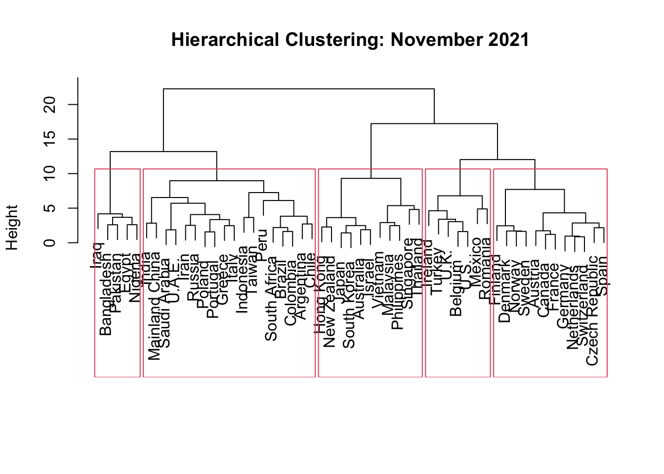

cluster_11 <- cutree(hc_11, k = 5)
cluster_11

 [1] 1 2 3 4 5 1 3 1 1 3 3 4 3 3 3 1 2 1 1 1 4 5 2 1 2 1 2 5 3 2 4 3 4 1 2 1 1 5
[39] 1 1 2 1 2 3 3 3 1 2 5 1 5 5 2

Question 1.2: Interpreting the November Dendrogram

Show answer

The November dendrogram suggests that several countries are quite different from most others. In particular, countries such as Nigeria, Pakistan, Bangladesh, Egypt, and Iraq form a small group that separates from many of the higher-income and more highly vaccinated countries. This indicates that their COVID resilience profiles were relatively different from the rest of the sample.

Some clusters look more compact than others. For example, the cluster containing many advanced economies such as Ireland, Spain, Denmark, Finland, Norway, France, Switzerland, Canada, Germany, and the United States is relatively large but internally similar in terms of healthcare coverage, development level, vaccination-related measures, and travel-related variables. The smaller cluster containing Bangladesh, Pakistan, Egypt, Iraq, and Nigeria is also clearly separated from the others.

Overall, the dendrogram suggests that country similarity in November 2021 was strongly related to vaccination coverage, healthcare/development indicators, case fatality patterns, mobility, and travel reopening measures.

Question 1.3: Cluster Membership Table for November

Create a table showing at least the following:

country
Bloomberg rank
cluster membership

Sort the table by cluster and then by rank.

Show answer

cluster_table_11 <- bloomberg_11 |>
  mutate(cluster = cluster_11) |>
  select(country, RANK, cluster) |>
  arrange(cluster, RANK)

cluster_table_11

# A tibble: 53 × 3
   country         RANK cluster
   <chr>          <dbl>   <int>
 1 U.A.E.             3       1
 2 Chile              8       1
 3 Saudi Arabia      15       1
 4 Portugal          18       1
 5 Greece            23       1
 6 Italy             24       1
 7 Colombia          27       1
 8 Mainland China    28       1
 9 Brazil            31       1
10 Poland            33       1
# ℹ 43 more rows

Question 1.4: PCA for November

Using the standardized November data:

Run PCA.
Print the PCA summary.
Create a scree plot.
Display the loading matrix.
Obtain the principal component scores.

Show answer

X <- scale(bloomberg_11_num)
pca_11 <- prcomp(X, scale. = FALSE)

summary(pca_11)

Importance of components:
                          PC1    PC2    PC3    PC4     PC5     PC6     PC7
Standard deviation     1.6821 1.4348 1.2063 1.1281 0.99296 0.84462 0.72826
Proportion of Variance 0.2572 0.1872 0.1323 0.1157 0.08963 0.06485 0.04822
Cumulative Proportion  0.2572 0.4444 0.5767 0.6924 0.78200 0.84686 0.89507
                           PC8     PC9    PC10    PC11
Standard deviation     0.64241 0.59495 0.55486 0.28225
Proportion of Variance 0.03752 0.03218 0.02799 0.00724
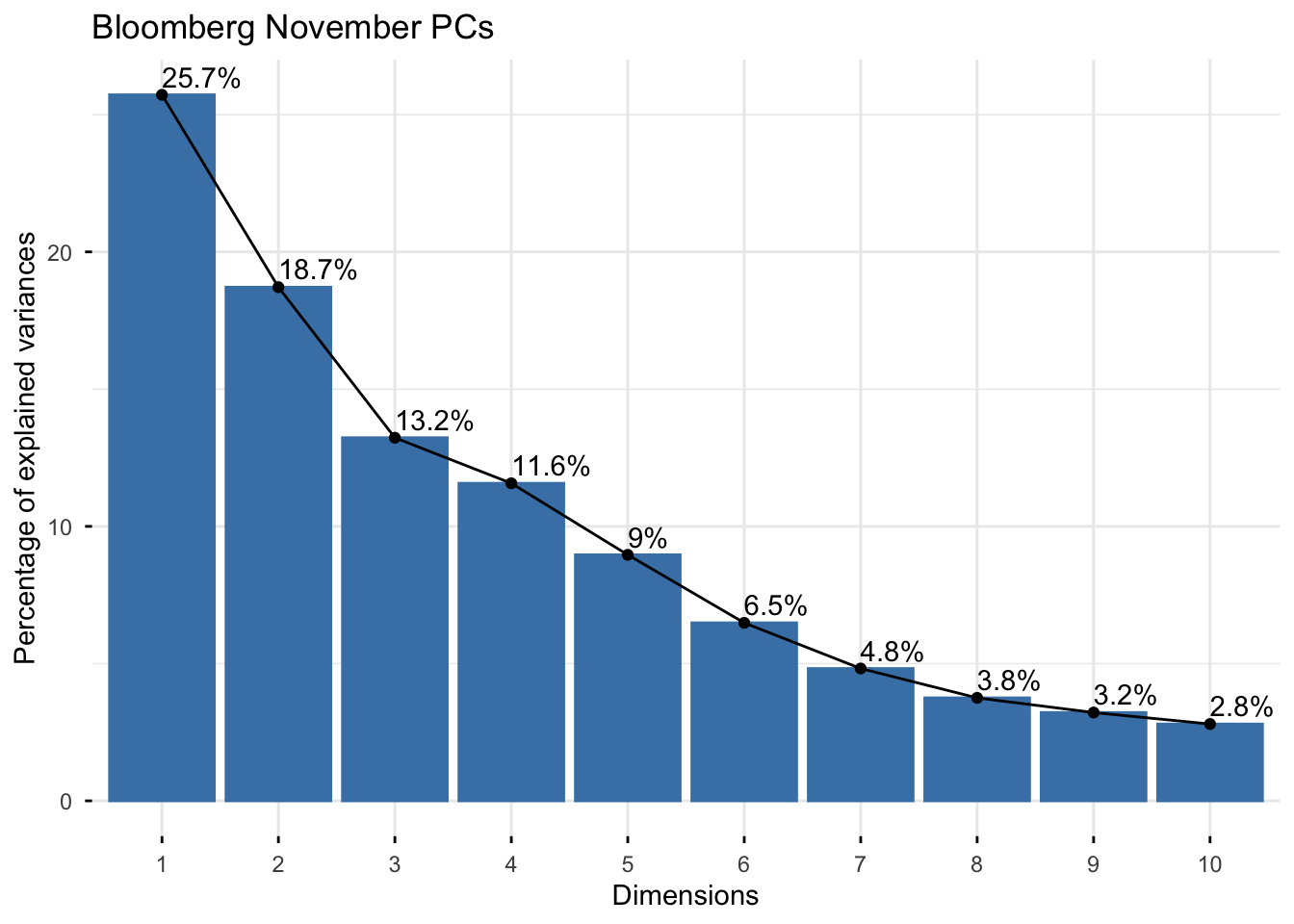
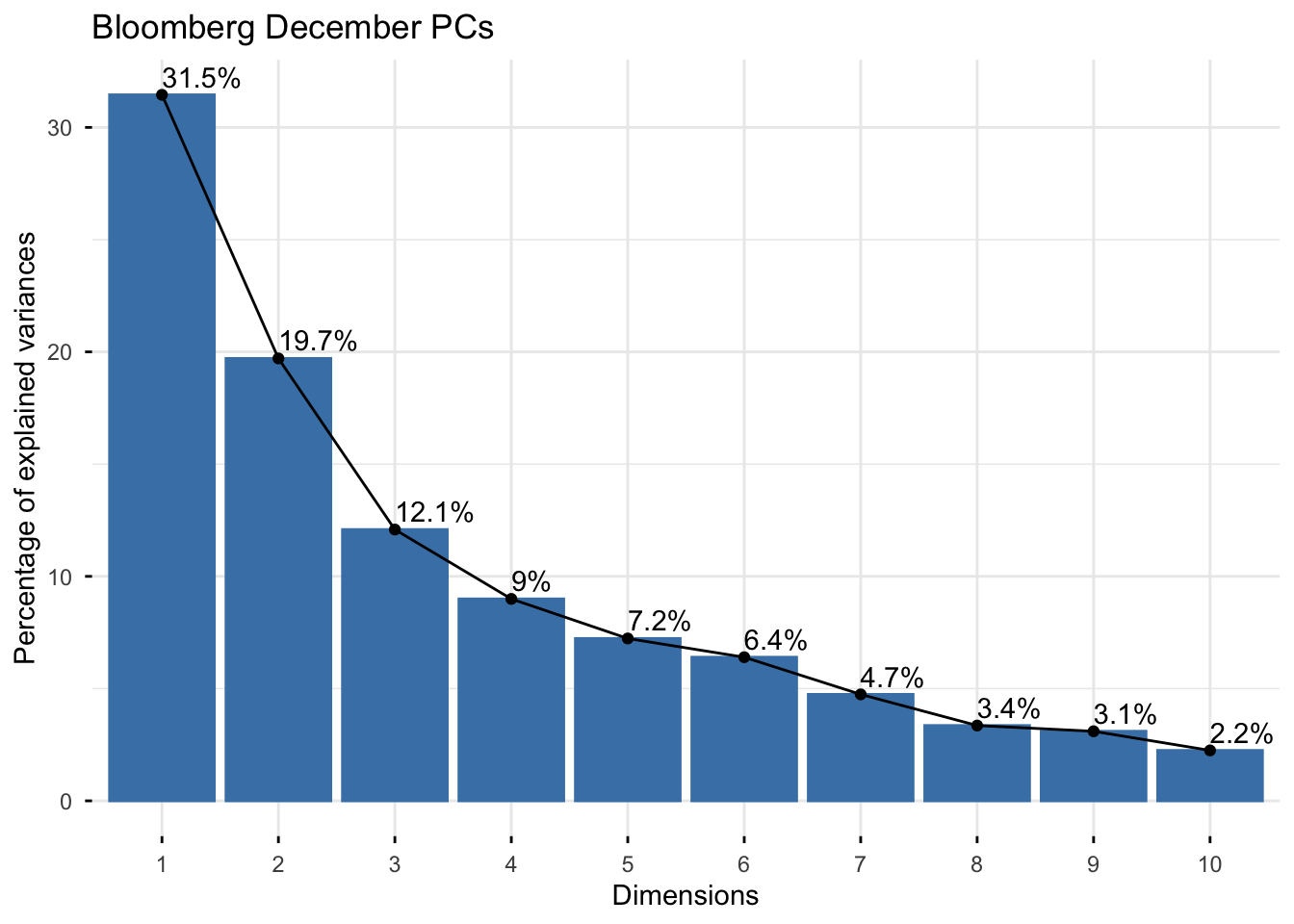
Cumulative Proportion  0.93259 0.96477 0.99276 1.00000

# Scree plot using factoextra
fviz_eig(
  pca_11,
  addlabels = TRUE,
  ncp = 10,
  main = "Bloomberg November PCs"
)

loadings_11 <- t(round(pca_11$rotation, 2))[1:3, ]
loadings_11

    LOCKDOWN SEVERITY FLIGHT CAPACITY VACCINATED TRAVEL ROUTES
PC1              0.03            0.19                     0.08
PC2             -0.07            0.42                     0.45
PC3              0.52           -0.16                    -0.39
    1-MONTH CASES PER 100,000 3-MONTH CASE FATALITY RATE
PC1                     -0.32                       0.34
PC2                      0.34                       0.09
PC3                      0.15                       0.30
    TOTAL DEATHS PER 1 MILLION POSITIVE TEST RATE COMMUNITY MOBILITY
PC1                      -0.04              -0.04               0.41
PC2                       0.51               0.34               0.10
PC3                       0.14               0.15              -0.39
    2021 GDP GROWTH FORECAST UNIVERSAL HEALTHCARE COVERAGE
PC1                    -0.07                         -0.53
PC2                     0.31                          0.04
PC3                     0.42                         -0.18
    HUMAN DEVELOPMENT INDEX
PC1                   -0.53
PC2                    0.00
PC3                   -0.18

scores_11 <- as_tibble(predict(pca_11, X))
scores_11

# A tibble: 53 × 11
     PC1    PC2    PC3     PC4    PC5    PC6      PC7    PC8    PC9   PC10  PC11
   <dbl>  <dbl>  <dbl>   <dbl>  <dbl>  <dbl>    <dbl>  <dbl>  <dbl>  <dbl> <dbl>
 1  15.7  10.3   24.5   26.6    23.2   -7.84  -7.76   -23.6  -22.4    3.14  4.37
 2 -18.8 -18.3  -19.3   -5.55  -16.1    7.53  -1.90     9.31  22.6    3.93 -8.19
 3 -17.5 -16.5  -24.2   -4.35  -24.3    4.49  -0.198   12.2   24.5    4.01 -7.88
 4  26.9  -1.68  -4.80   4.21    4.51   2.41  -0.443   -4.71  -6.94  18.6  14.6 
 5 -20.9   1.75 -11.1  -10.2   -24.1  -10.7   -6.78    23.2   10.5  -15.8  -9.71
 6  21.0   4.38  10.2    3.83   22.6    8.09   8.10   -16.8  -16.6   12.0   8.04
 7 -14.7  -6.76 -10.5    0.343 -15.2   -1.65  -2.85     7.59  13.1   -3.05 -7.33
 8  21.6  31.8   53.6   52.1    32.2  -28.6  -14.6    -39.0  -39.7  -13.1   6.61
 9  24.0  19.8   32.0   26.0    26.6  -11.1   -2.51   -26.3  -28.8   -1.12  9.52
10 -14.2 -15.9  -25.1  -13.0   -19.4    7.51  -0.0777  16.4   19.4    5.80 -6.58
# ℹ 43 more rows

Question 1.5: PCA Score Plot for November

Create a scatter plot of PC1 vs PC2.

Label points with country names, or with a combined label such as rank and country.
Color points by the 5-cluster membership obtained from hierarchical clustering.

Show answer

pca_plot_11 <- scores_11 |>
  mutate(
    country = bloomberg_11$country,
    rank = bloomberg_11$RANK,
    cluster = as.factor(cluster_11),
    label = paste(rank, country)
  )

ggplot(pca_plot_11, aes(x = PC1, y = PC2, color = cluster)) +
  geom_point(size = 3, alpha = 0.8) +
  geom_text_repel(aes(label = label), max.overlaps = 60, size = 3) +
  labs(
    title = "PCA Score Plot: November 2021",
    x = "PC1",
    y = "PC2",
    color = "Cluster"
  ) +
  theme_minimal()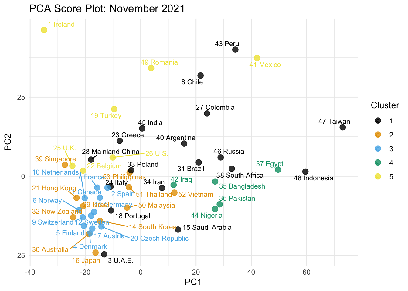

Question 1.6: Interpreting the November PCA Results

Show answer

For November, PC1 explains about 25.7% of the total variance and PC2 explains about 18.7%. Together, the first two principal components explain about 44.4% of the total variation in the standardized resilience variables.

PC1 mainly contrasts countries with stronger healthcare/development profiles against countries with weaker profiles. In the loading matrix, UNIVERSAL HEALTHCARE COVERAGE and HUMAN DEVELOPMENT INDEX have large negative loadings, while COMMUNITY MOBILITY and 3-MONTH CASE FATALITY RATE have positive loadings. Therefore, countries with lower PC1 scores tend to have stronger healthcare and development indicators, while countries with higher PC1 scores tend to have weaker healthcare/development profiles and higher mobility or fatality-rate-related values.

PC2 mainly reflects travel reopening and measured COVID burden. It has relatively large positive loadings on FLIGHT CAPACITY, VACCINATED TRAVEL ROUTES, TOTAL DEATHS PER 1 MILLION, 1-MONTH CASES PER 100,000, and POSITIVE TEST RATE. Therefore, countries with higher PC2 scores tend to have more travel activity and/or heavier measured COVID burden.

In the score plot, countries such as Ireland, the Netherlands, Switzerland, Finland, Sweden, Norway, Canada, Denmark, and Austria appear on the lower-PC1 side, suggesting stronger healthcare/development profiles. Countries such as Indonesia, Taiwan, Egypt, South Africa, Bangladesh, Pakistan, and Nigeria appear on the higher-PC1 side, suggesting weaker profiles on those dimensions. Countries such as Ireland, Mexico, Peru, Romania, Chile, and Colombia appear high on PC2, while Japan, U.A.E., Denmark, Finland, Sweden, and Switzerland appear low on PC2.

The PCA plot broadly supports the clustering result because countries in the same hierarchical cluster tend to appear near one another in the PC1-PC2 space. However, the PCA plot only shows the first two principal components, so it cannot perfectly reproduce the full clustering result based on all standardized variables.

Part 2. December 2021 Analysis

Question 2.1: Hierarchical Clustering for December

Repeat the hierarchical clustering analysis for the December data.

Use the same general steps as in Part 1, again using 5 clusters.

Show answer

dist_12 <- dist(bloomberg_12_scaled, method = "euclidean")

hc_12 <- hclust(dist_12, method = "ward.D")

plot(
  hc_12,
  labels = bloomberg_12$country,
  main = "Hierarchical Clustering: December 2021",
  xlab = "",
  sub = ""
)
rect.hclust(hc_12, k = 5)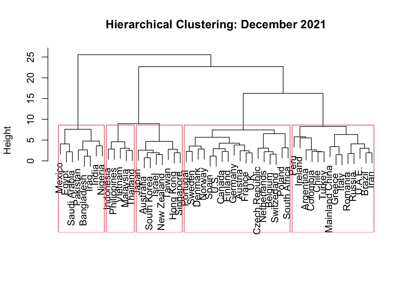

cluster_12 <- cutree(hc_12, k = 5)
cluster_12

 [1] 1 2 3 4 3 1 3 1 1 3 3 4 3 3 3 1 2 4 5 1 4 1 2 1 2 1 5 4 3 2 4 3 4 1 5 3 3 1
[39] 1 4 2 3 2 3 3 3 2 5 1 1 3 3 5

Question 2.2: Interpreting the December Dendrogram

Show answer

The December dendrogram again shows that some countries are unusually different from the rest. Nigeria, Pakistan, Bangladesh, Iraq, and Egypt remain part of a low-resilience-profile group, although Mexico and India are also grouped near this part of the structure in the 5-cluster solution.

Several high-income countries appear similar to one another, including Ireland, Finland, Canada, Spain, Sweden, the United Kingdom, Denmark, the United States, France, Portugal, Norway, Switzerland, Austria, Belgium, the Netherlands, Germany, and the Czech Republic. Another compact group includes South Korea, Australia, Singapore, Israel, Hong Kong, New Zealand, Taiwan, and Japan.

Compared with November, the December structure is similar in broad terms, but not identical. The high-income/development cluster remains clear, and the lower-healthcare/development cluster remains clear. However, several countries shift cluster membership as COVID conditions, travel reopening measures, vaccine dose measures, and case rates changed between November and December.

Question 2.3: Cluster Membership Table for December

Create a table showing:

country
Bloomberg rank
cluster membership

Sort the table by cluster and then by rank.

Show answer

cluster_table_12 <- bloomberg_12 |>
  mutate(cluster = cluster_12) |>
  select(country, RANK, cluster) |>
  arrange(cluster, RANK)

cluster_table_12

# A tibble: 53 × 3
   country         RANK cluster
   <chr>          <dbl>   <int>
 1 Chile              1       1
 2 Ireland            2       1
 3 U.A.E.             3       1
 4 Colombia           6       1
 5 Turkey             7       1
 6 Iran              14       1
 7 Argentina         19       1
 8 Mainland China    28       1
 9 Italy             32       1
10 Greece            35       1
# ℹ 43 more rows

Question 2.4: PCA for December

Repeat the PCA analysis for the December data.

Include:

PCA summary
Scree plot
Loading matrix
Principal component scores

Show answer

X <- scale(bloomberg_12_num)
pca_12 <- prcomp(X, scale. = FALSE)

summary(pca_12)

Importance of components:
                          PC1    PC2    PC3     PC4     PC5     PC6     PC7
Standard deviation     1.8600 1.4724 1.1530 0.99474 0.89195 0.83895 0.72230
Proportion of Variance 0.3145 0.1971 0.1209 0.08995 0.07233 0.06399 0.04743
Cumulative Proportion  0.3145 0.5116 0.6325 0.72242 0.79474 0.85873 0.90616
                           PC8    PC9    PC10    PC11
Standard deviation     0.60753 0.5839 0.49711 0.27410
Proportion of Variance 0.03355 0.0310 0.02247 0.00683
Cumulative Proportion  0.93971 0.9707 0.99317 1.00000

# Scree plot using factoextra
fviz_eig(
  pca_12,
  addlabels = TRUE,
  ncp = 10,
  main = "Bloomberg December PCs"
)

loadings_12 <- t(round(pca_12$rotation, 2))[1:3, ]
loadings_12

    LOCKDOWN SEVERITY FLIGHT CAPACITY VACCINATED TRAVEL ROUTES
PC1              0.15           -0.09                    -0.04
PC2              0.09            0.49                     0.51
PC3              0.42            0.09                    -0.29
    1-MONTH CASES PER 100,000 3-MONTH CASE FATALITY RATE
PC1                      0.39                      -0.37
PC2                      0.23                       0.17
PC3                     -0.33                       0.07
    TOTAL DEATHS PER 1 MILLION POSITIVE TEST RATE COMMUNITY MOBILITY
PC1                       0.12               0.19              -0.41
PC2                       0.49               0.26               0.07
PC3                       0.25              -0.49              -0.14
    2021 GDP GROWTH FORECAST UNIVERSAL HEALTHCARE COVERAGE
PC1                     0.07                          0.48
PC2                     0.29                         -0.06
PC3                     0.54                          0.06
    HUMAN DEVELOPMENT INDEX
PC1                    0.47
PC2                   -0.10
PC3                    0.06

scores_12 <- as_tibble(predict(pca_12, X))
scores_12

# A tibble: 53 × 11
      PC1    PC2     PC3     PC4    PC5      PC6    PC7    PC8    PC9   PC10
    <dbl>  <dbl>   <dbl>   <dbl>  <dbl>    <dbl>  <dbl>  <dbl>  <dbl>  <dbl>
 1   1.89   9.80  17.6   -15.8     5.55 -19.6      7.34  -3.76 -12.6    6.90
 2  15.5  -16.3   -6.25    0.516  21.8    1.17    -9.93   4.72  18.3  -17.3 
 3  21.1  -17.5   -3.56    2.52   19.9   -0.0902 -10.4   -2.58  18.4  -25.3 
 4 -29.4    3.71  -1.28    2.67   -8.09  13.5     -3.55   1.30   3.50  17.6 
 5  26.6   -3.85  -5.45   -1.85   26.5  -23.3      4.99   6.83   9.49 -23.5 
 6 -24.4    9.88  -0.255   5.18  -28.0   18.8      2.53  -1.84 -12.7   23.2 
 7  14.6  -10.1   -4.91    1.01   15.4   -1.76    -4.70   3.30  11.5  -14.6 
 8  10.5   19.9   47.8   -37.4    29.2  -40.6     17.7  -15.5  -16.9    1.85
 9 -12.9   22.2   28.8   -18.3    -2.58 -12.0     15.4  -10.6  -20.0   18.3 
10  15.5  -15.3  -22.5    12.1    11.7   -0.0384  -7.99  11.0   17.7  -19.3 
# ℹ 43 more rows
# ℹ 1 more variable: PC11 <dbl>

Question 2.5: PCA Score Plot for December

Create a scatter plot of PC1 vs PC2 for December.

Label points clearly.
Color points by the December cluster membership.

Show answer

pca_plot_12 <- scores_12 |>
  mutate(
    country = bloomberg_12$country,
    rank = bloomberg_12$RANK,
    cluster = as.factor(cluster_12),
    label = paste(rank, country)
  )

ggplot(pca_plot_12, aes(x = PC1, y = PC2, color = cluster)) +
  geom_point(size = 3, alpha = 0.8) +
  geom_text_repel(aes(label = label), max.overlaps = 60, size = 3) +
  labs(
    title = "PCA Score Plot: December 2021",
    x = "PC1",
    y = "PC2",
    color = "Cluster"
  ) +
  theme_minimal()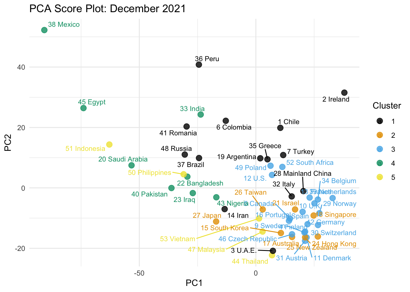

Question 2.6: Interpreting the December PCA Results

Show answer

For December, PC1 explains about 31.5% of the total variance and PC2 explains about 19.7%. Together, PC1 and PC2 explain about 51.2% of the variation in the standardized variables.

PC1 represents a broad healthcare, development, and COVID-condition dimension. It has large positive loadings on UNIVERSAL HEALTHCARE COVERAGE, HUMAN DEVELOPMENT INDEX, and 1-MONTH CASES PER 100,000, and negative loadings on COMMUNITY MOBILITY and 3-MONTH CASE FATALITY RATE. Therefore, countries with higher PC1 scores tend to have stronger healthcare/development profiles, while countries with lower PC1 scores tend to have weaker healthcare/development profiles and higher community mobility or fatality-rate-related values.

PC2 mainly reflects travel reopening and measured COVID burden. It has large positive loadings on VACCINATED TRAVEL ROUTES, FLIGHT CAPACITY, TOTAL DEATHS PER 1 MILLION, 2021 GDP GROWTH FORECAST, POSITIVE TEST RATE, and 1-MONTH CASES PER 100,000. Therefore, countries with higher PC2 scores tend to have more travel activity and/or heavier measured COVID burden.

In the score plot, countries such as the U.K., Norway, Denmark, Switzerland, Germany, Belgium, the Netherlands, and Ireland appear on the higher-PC1 side, suggesting stronger healthcare/development profiles. Countries such as Mexico, Egypt, Indonesia, Saudi Arabia, Pakistan, Bangladesh, and Iraq appear on the lower-PC1 side, suggesting weaker profiles on those dimensions. Countries such as Mexico, Peru, Ireland, Egypt, India, Chile, and Colombia appear high on PC2, while Thailand, U.A.E., Malaysia, Vietnam, Japan, Austria, New Zealand, and Denmark appear low on PC2.

The PCA result aligns reasonably well with the 5-cluster solution. Countries in the same cluster are often grouped near each other in the score plot. Still, the alignment is not perfect because hierarchical clustering uses all standardized variables, while the PCA score plot shows only PC1 and PC2.

Part 3. Comparing November and December

Question 3.1

Compare the November and December clustering results.

Discuss at least the following:

Did some countries appear to move into a different cluster?
Did the overall cluster structure seem stable across months, or did it change noticeably?
What might explain any differences you observe?

Show answer

Some countries appear to move across clusters between November and December, although the movements are not drastic for most countries. For example, Mexico, Turkey, and some Eastern European or Latin American countries shift their relative positions. Some East Asian and Oceania countries, such as Taiwan, Australia, Japan, and New Zealand, also change their locations slightly in the PCA score plots.

Overall, the cluster structure is fairly stable across the two months. In both November and December, there is a clear separation between:

high-income countries with stronger healthcare and development indicators, and
countries with weaker healthcare/development profiles.

However, the exact cluster membership changes somewhat across months.

These differences may be explained by changing COVID conditions in late 2021. Variables such as cases, deaths, positivity rates, mobility, lockdown severity, and travel reopening can change from month to month. Since clustering is based on the full standardized profile of each country, even moderate changes across several variables can move a country into a different cluster.

Question 3.2

Compare the November and December PCA results.

Discuss at least the following:

Was the proportion of variance explained by PC1 and PC2 similar across months?
Did the interpretation of PC1 and PC2 remain similar, or did it change?
Were the same countries extreme in both months?

Show answer

The proportion of variance explained by the first two principal components is similar but slightly higher in December. In November, PC1 and PC2 explain about 44.4% of the total variance, while in December they explain about 51.2%. This suggests that the first two components summarize the structure of the December data somewhat more clearly.

The interpretation of PC1 and PC2 remains broadly similar across months. In both months, PC1 is mainly related to healthcare and development indicators, especially UNIVERSAL HEALTHCARE COVERAGE and HUMAN DEVELOPMENT INDEX. In November, stronger healthcare/development profiles are associated with lower PC1 values, while in December they are associated with higher PC1 values. This sign difference does not change the meaning, because the direction of a principal component can be reversed.

PC2 in both months reflects a mix of travel reopening and measured COVID burden, including variables such as FLIGHT CAPACITY, VACCINATED TRAVEL ROUTES, cases, deaths, and positivity rates. Higher PC2 values generally indicate more travel activity and/or heavier measured COVID burden.

Many of the same countries remain extreme across months. Countries such as Nigeria, Pakistan, Bangladesh, Egypt, and Indonesia tend to appear on the weaker healthcare/development side of PC1. High-income countries such as the U.K., Norway, Denmark, Switzerland, Belgium, the Netherlands, and Ireland tend to appear on the stronger side. Countries such as Mexico and Peru are relatively extreme on PC2, suggesting stronger association with the COVID-burden or travel-activity dimension.

Question 3.3

Write a short concluding paragraph summarizing what you learned from the clustering and PCA analyses of the Bloomberg COVID Resilience Rankings.

Show answer

The clustering and PCA analyses show that countries’ COVID resilience profiles in late 2021 were driven by multiple dimensions rather than a single factor. The most important contrast is between countries with stronger healthcare systems and higher human development and countries with weaker profiles in these areas. A second important dimension captures differences in travel activity and measured COVID burden, including cases, deaths, and positivity rates. While the overall structure is fairly stable across November and December, some countries shift because pandemic conditions and policy responses changed over time. Overall, these unsupervised learning methods provide a useful way to summarize complex country-level patterns without relying directly on the Bloomberg resilience score.