Homework 1

Linear Regression · Quarto Blogging

Directions

• Submit your Quarto document for Part 1 to Brightspace using this filename format:

  • danl-320-hw1-LASTNAME-FIRSTNAME.qmd
    (e.g., danl-320-hw1-choe-byeonghak.qmd)

• Due: February 11, 2026, 3:15 PM (ET)

• Questions? Email Byeong-Hak bchoe@geneseo.edu.

Required R Packages

library(tidyverse)
library(stargazer)
library(broom)

Part 1. Linear Regression

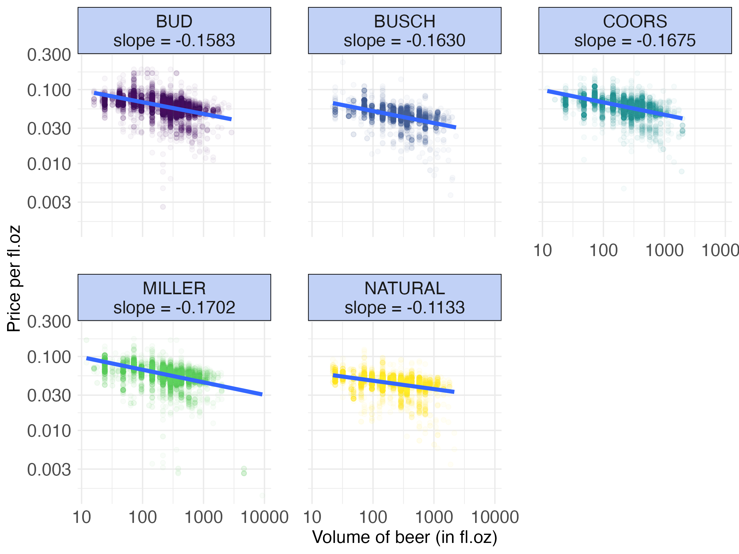
Consider the beer_markets data:

library(tidyverse)

beer_markets <- read_csv(
  "https://bcdanl.github.io/data/beer_markets_all_cleaned.csv"
)

Variable Description

Variable Name	Description
household	Unique identifier for household
X_purchase_desc	Description of beer purchase
quantity	Number of beer packages purchased
brand	Brand of beer purchased
dollar_spent	Total amount spent on the purchase
beer_floz	Total volume of beer purchased (in fluid ounces)
price_floz	Price per fluid ounce of beer
container	Type of beer container (e.g., CAN, BOTTLE)
promo	Indicates if the purchase was part of a promotion (TRUE/FALSE)
region	Geographic region of purchase
marital	Marital status of household head
income	Income level of the household
age	Age group of household head
employment	Employment status of household head
degree	Education level of household head
occupation	Occupation category of household head
ethnic	Ethnicity of household head
microwave	Indicates if the household owns a microwave (TRUE/FALSE)
dishwasher	Indicates if the household owns a dishwasher (TRUE/FALSE)
tvcable	Type of television subscription (e.g., basic, premium)
singlefamilyhome	Indicates if the household is a single-family home (TRUE/FALSE)
npeople	Number of people in the household

Question 1 — Filter the data (containers)

Create a data frame that keeps only observations where container is:

• "CAN" or
• "NON_REFILLABLE_BOTTLE"

Requirements:

• Name your filtered data frame beer_sub.
• Report the number of observations in beer_sub.
• Report a frequency table of container in beer_sub.

Show answer

With %in% operator

beer_sub <- beer_markets |> 
  filter(container %in% c("CAN", "NON_REFILLABLE_BOTTLE"))

With OR (|) operator

#| eval: false

beer_sub <- beer_markets |> 
  filter(container == "CAN" | container == "NON_REFILLABLE_BOTTLE")

Question 2 — Train/test split

Split beer_sub into two data frames:

• Training set (beer_train): about 67% of observations
• Test set (beer_test): the remaining observations

Requirements:

• Use a random seed for reproducibility (you choose the seed).
• Report nrow(beer_train) and nrow(beer_test).
• Briefly explain why we keep a test set.

Show answer

With runif(n())

# 1) reproducible split
set.seed(1)  # you can choose any seed

# 2) sample row indices
beer_sub <- beer_sub |> 
  mutate(rnd = runif(n())) # n() number of random numbers from Unif(0,1) are drawn

# Setting reference levels
beer_sub <- beer_sub |> 
  mutate(market = factor(market),
         market = fct_relevel(market, "BUFFALO-ROCHESTER"),
         brand = factor(brand),
         brand = fct_relevel(brand, "BUD_LIGHT")
         )

# 2-1) sample row indices for training (about 67%)
beer_train <- beer_sub |> 
  filter(rnd >= 0.33)

# 2-1) sample row indices for test (about 33%)
beer_test <- beer_sub |> 
  filter(rnd < 0.33)


# 3) report sizes
nrow(beer_train)

[1] 48322

nrow(beer_test)

[1] 23788

With sample.int(n)

#| eval: false

# 1) reproducible split
set.seed(1)  # you can choose any seed

# 2) sample row indices for training (about 67%)
n <- nrow(beer_sub)
train_idx <- sample.int(n = n, size = round(0.67 * n), replace = FALSE)

beer_train <- beer_sub[train_idx, ]
beer_test  <- beer_sub[-train_idx, ]

# 3) report sizes
nrow(beer_train)

[1] 48314

nrow(beer_test)

[1] 23796

Questions 3–8 (Regression models)

You will estimate three linear regression models for:

• Outcome: \(\log(\text{price\_floz})\)

Reference levels (required):

• Set "BUD_LIGHT" as the reference level for brand.
• Set "BUFFALO-ROCHESTER" as the reference level for market.
  • There are \(N+1\) distinct categories in market:

Model 1

\[ \begin{aligned} \log(\text{price\_floz}) = &\ \beta_{0} + \sum_{i=1}^{N} \beta_{i} \,\text{market}_{i} + \sum_{j=N+1}^{N+4} \beta_{j} \,\text{brand}_{j} + \beta_{N+5} \,\text{container\_CAN} \\ &\,+\, \beta_{N+6} \log(\text{beer\_floz}) + \epsilon \end{aligned} \]

Model 2 (brand-specific volume sensitivity)

\[ \begin{aligned} \log(\text{price\_floz}) \,=\, & \beta_{0} \,+\, \sum_{i=1}^{N}\beta_{i}\,\text{market}_{i} \,+\, \sum_{j=N+1}^{N+4}\beta_{j}\,\text{brand}_{j} \,+\, \beta_{N+5}\,\text{container\_CAN} \\ &\,+\, \beta_{N+6}\log(\text{beer\_floz})\\ &\,+\, \sum_{j=N+1}^{N+4}\beta_{j\times\text{beer\_floz}}\,\text{brand}_{j}\times \log(\text{beer\_floz})\\ &\,+\, \epsilon \end{aligned} \]

Model 3 (promo + brand-specific promo effects)

\[ \begin{aligned} \log(\text{price\_floz}) \,=\, & \beta_{0} \,+\, \sum_{i=1}^{N}\beta_{i}\,\text{market}_{i} \,+\, \sum_{j=N+1}^{N+4}\beta_{j}\,\text{brand}_{j} \,+\, \beta_{N+5}\,\text{container\_CAN} \\ &\,+\, \beta_{N+6}\log(\text{beer\_floz})\\ &\,+\, \beta_{N+7}\,\text{promo} \times\log(\text{beer\_floz}) \\ &\,+\, \sum_{j=N+1}^{N+4}\beta_{j\times\text{beer\_floz}}\,\text{brand}_{j}\times \log(\text{beer\_floz})\\ &\,+\, \sum_{j=N+1}^{N+4}\beta_{j\times\text{promo}}\,\text{brand}_{j}\times \text{promo}\\ &\,+\, \sum_{j=N+1}^{N+4}\beta_{j\times\text{promo}\times\text{beer\_floz}}\,\text{brand}_{j}\times \text{promo}\times \log(\text{beer\_floz})\\ &\,+\, \epsilon \end{aligned} \]

---

How to Interpret \(\beta\) Coefficients in Linear Regression

Assume \(d\) is a dummy variable (0/1). Interpretations are ceteris paribus (holding other variables constant).

1) Level–Level Model

\[y = \beta_1 x_1 + \beta_2 d\]

Interpretation

• \(\beta_1\): a one-unit increase in \(x_1\) changes \(y\) by \(\beta_1\) units.
  • “If \(x_1\) increases by 1, expected \(y\) changes by \(\beta_1\).”
• \(\beta_2\) (dummy): changing \(d\) from 0 to 1 changes \(y\) by \(\beta_2\) units.
  • “The \(d=1\) group has \(y\) that is \(\beta_2\) higher/lower than the \(d=0\) group.”

2) Log–Level Model (Semi-log)

\[\log(y) = \beta_1 x_1 + \beta_2 d\]

Interpretation (for \(x_1\))

• \(\beta_1\): a one-unit increase in \(x_1\) changes \(y\) by approximately \(100\beta_1\%\).
  • More accurate:
  • \(\%\Delta y = 100\,(e^{\beta_1}-1)\)

Interpretation (for dummy \(d\))

• \(\beta_2\): switching from \(d=0\) to \(d=1\) changes \(y\) by:
• \(\%\Delta y = 100\,(e^{\beta_2}-1)\)
  • “The \(d=1\) group has \(y\) that is \(100(e^{\beta_2}-1)\%\) higher/lower than the \(d=0\) group.”

3) Log–Log Model (Elasticity Model)

\[\log(y) = \beta_1 \log(x_1) + \beta_2 d\]

Interpretation (for \(\log(x_1)\))

• \(\beta_1\) is an elasticity:
  • a 1% increase in \(x_1\) is associated with a \(\beta_1\%\) change in \(y\).
    
  • “If \(x_1\) rises by 1%, expected \(y\) changes by \(\beta_1\%\).”

Interpretation (for dummy \(d\))

• \(\beta_2\): switching from \(d=0\) to \(d=1\) changes \(y\) by:
• \(\%\Delta y = 100\,(e^{\beta_2}-1)\)

Quick Summary

• Level–Level: \(\beta\) = units of \(y\) per 1 unit of \(x\)
  
• Log–Level: \(\beta \approx\) % change in \(y\) per 1 unit of \(x\)
  
• Log–Log: \(\beta\) = % change in \(y\) per 1% change in \(x\) (elasticity)
  
• Dummy in \(\log(y)\): percent difference is \(100(e^{\beta}-1)\%\)

---

Question 3 — Model intuition (conceptual)

For each model, explain in plain English:

• What is the model trying to capture?
• What kinds of differences across markets and brands are allowed?
• How does the model treat the relationship between volume (beer_floz) and price (price_floz)?
• What new flexibility is added when moving from Model 1 → 2 → 3?

Show answer

• Model 1

\[ \begin{align} \log(\text{price\_per\_floz}) = &\ \beta_{0} + \sum_{i=1}^{N} \beta_{i} \,\text{market}_{i} + \sum_{j=N+1}^{N+4} \beta_{j} \,\text{brand}_{j} + \beta_{N+5} \,\text{container\_{CAN}} \\ &\,+\, \beta_{N+6} \log(\text{beer\_floz}) + \epsilon \end{align} \]

• One-Size-Fits-All Elasticity
  • Assumes that every beer—whether Budweiser or value-priced Natural—shares an identical volume elasticity.
  • The entire beer is treated as a homogeneous commodity. A 10 % increase in price invariably yields, for example, a 5 % reduction in sales, regardless of brand identity or promotional activity.
  • While straightforward to estimate, this specification overlooks differences in pricing power across brands, positioning, and promotional responsiveness, leading to underpricing of premium favorites (e.g., Bud, Coors, Miller) and overpricing of bargain brands (e.g., Busch, Natural).
• Model 2

\[ \begin{align} \log(\text{price\_per\_floz}) \,=\, & \beta_{0} \,+\, \sum_{i=1}^{N}\beta_{i}\,\text{market}_{i} \,+\, \sum_{j=N+1}^{N+4}\beta_{j}\,\text{brand}_{j} \,+\, \beta_{N+5}\,\text{container\_{CAN}} \\ &\,+\, \beta_{N+6}\log(\text{beer\_floz})\\ &\,+\, \sum_{j=N+1}^{N+4}\beta_{j\times\text{beer\_floz}}\,\text{brand}_{j}\times \log(\text{beer\_floz})\\ &\,+\, \epsilon \end{align} \]

• Brand-Specific Elasticity (No Promotional Effect)
  • Allows Bud, Coors, Miller, Busch, and Natural each to exhibit its own volume elasticity, yet treats promotion and no-promotion identically.
  • The model imposes a constant sensitivity irrespective of whether the price is part of a “Happy Hour” or standard offering.
    • This approach captures variation in the degrees of sensitiveness across brands, but it fails to account for the additional demand shifts induced by promotions.
• Model 3

\[ \begin{align} \log(\text{price\_per\_floz}) \,=\, & \beta_{0} \,+\, \sum_{i=1}^{N}\beta_{i}\,\text{market}_{i} \,+\, \sum_{j=N+1}^{N+4}\beta_{j}\,\text{brand}_{j} \,+\, \beta_{N+5}\,\text{container\_{CAN}} \\ &\,+\, \beta_{N+6}\log(\text{beer\_floz})\\ &\,+\, \beta_{N+7}\,\text{promo} \times\log(\text{beer\_floz}) \\ &\,+\, \sum_{j=N+1}^{N+4}\beta_{j\times\text{beer\_floz}}\,\text{brand}_{j}\times \log(\text{beer\_floz})\\ &\,+\, \sum_{j=N+1}^{N+4}\beta_{j\times\text{promo}}\,\text{brand}_{j}\times \text{promo}\\ &\,+\, \sum_{j=N+1}^{N+4}\beta_{j\times\text{promo}\times\text{beer\_floz}}\,\text{brand}_{j}\times \text{promo}\times \log(\text{beer\_floz})\\ &\,+\, \epsilon \end{align} \]

• Brand * Promotion-Specific Elasticity
  • Estimates a distinct elasticity for each brand and for each brand’s promotional status (discounted vs. full price).
    • When Natural Light is on special, its demand becomes markedly more elastic—deal-seeking consumers flood in—whereas Bud devotees remain relatively insensitive to a buy-one-get-one offer. Each brand’s “promotion effect” is modeled uniquely.
    • This specification offers the greatest flexibility, supporting a dynamic pricing and promotional calendar that maximizes profitability by aligning strategies with each brand’s specific consumer responsiveness.

Question 4 — Estimate, predict, and evaluate

Using beer_train:

1. Fit Model 1, Model 2, and Model 3 using lm().
2. Provide a regression table or summary() output for each model.
3. Using beer_test, generate out-of-sample predictions:
   • predict \(\log(\text{price\_floz})\)
   • convert predictions back to price_floz using exp()
4. Evaluate predictive performance on beer_test:
   • report RMSE (required)

Requirements:

• Present results in a small table comparing Model 1–3 test RMSE.
• Briefly comment on which model predicts best and by how much.

Show answer

# Fit the models
m1 <- lm(data = beer_train,
         log(price_floz) ~ log(beer_floz) + brand + container + market)
m2 <- lm(data = beer_train,
         log(price_floz) ~ log(beer_floz) * brand + container + market)
m3 <- lm(data = beer_train,
         log(price_floz) ~ log(beer_floz) * brand * promo + container + market)


# Regression table
stargazer(m1, m2, m3, 
          type = "html", # which requires the code chunk option: `#| results: asis`
          digits = 4)  

	Dependent variable:
	log(price_floz)
	(1)	(2)	(3)
log(beer_floz)	-0.1412***	-0.1481***	-0.1442***
	(0.0012)	(0.0021)	(0.0023)
brandBUSCH_LIGHT	-0.2602***	-0.2163***	-0.1896***
	(0.0028)	(0.0219)	(0.0231)
brandCOORS_LIGHT	-0.0028	-0.0067	0.0018
	(0.0024)	(0.0182)	(0.0193)
brandMILLER_LITE	-0.0103***	0.0710***	0.1035***
	(0.0022)	(0.0166)	(0.0178)
brandNATURAL_LIGHT	-0.3184***	-0.6106***	-0.5438***
	(0.0025)	(0.0174)	(0.0186)
promo			-0.0786**
			(0.0368)
containerNON_REFILLABLE_BOTTLE	0.0522***	0.0509***	0.0522***
	(0.0019)	(0.0019)	(0.0019)
marketALBANY	0.0302**	0.0322***	0.0235*
	(0.0125)	(0.0125)	(0.0124)
marketATLANTA	0.0868***	0.0855***	0.0805***
	(0.0101)	(0.0100)	(0.0099)
marketBALTIMORE	0.0983***	0.1015***	0.0901***
	(0.0133)	(0.0132)	(0.0131)
marketBIRMINGHAM	0.1274***	0.1340***	0.1290***
	(0.0103)	(0.0103)	(0.0102)
marketBOSTON	0.1307***	0.1308***	0.1265***
	(0.0109)	(0.0108)	(0.0107)
marketCHARLOTTE	0.0284***	0.0249**	0.0328***
	(0.0101)	(0.0100)	(0.0100)
marketCHICAGO	-0.0044	-0.0096	-0.0047
	(0.0095)	(0.0095)	(0.0094)
marketCINCINNATI	0.0849***	0.0797***	0.0768***
	(0.0101)	(0.0100)	(0.0100)
marketCLEVELAND	0.0663***	0.0618***	0.0567***
	(0.0102)	(0.0101)	(0.0100)
marketCOLUMBUS	0.0750***	0.0720***	0.0719***
	(0.0095)	(0.0095)	(0.0094)
marketDALLAS	0.2110***	0.2208***	0.2241***
	(0.0094)	(0.0094)	(0.0093)
marketDENVER	0.1328***	0.1307***	0.1413***
	(0.0109)	(0.0109)	(0.0108)
marketDES_MOINES	0.1380***	0.1353***	0.1281***
	(0.0112)	(0.0111)	(0.0110)
marketDETROIT	0.0904***	0.0870***	0.0877***
	(0.0096)	(0.0096)	(0.0095)
marketEXURBAN_NJ	0.2309***	0.2273***	0.2175***
	(0.0161)	(0.0161)	(0.0160)
marketEXURBAN_NY	0.1146***	0.1118***	0.1024***
	(0.0220)	(0.0218)	(0.0217)
marketGRAND_RAPIDS	0.0906***	0.0862***	0.0833***
	(0.0113)	(0.0112)	(0.0111)
marketHARTFORD-NEW_HAVEN	0.1483***	0.1463***	0.1432***
	(0.0138)	(0.0137)	(0.0136)
marketHOUSTON	0.1217***	0.1189***	0.1216***
	(0.0097)	(0.0096)	(0.0095)
marketINDIANAPOLIS	0.0491***	0.0477***	0.0472***
	(0.0101)	(0.0101)	(0.0100)
marketJACKSONVILLE	0.1287***	0.1228***	0.1226***
	(0.0123)	(0.0123)	(0.0122)
marketKANSAS_CITY	0.0762***	0.0713***	0.0639***
	(0.0115)	(0.0115)	(0.0114)
marketLITTLE_ROCK	0.0976***	0.0935***	0.0883***
	(0.0127)	(0.0127)	(0.0126)
marketLOS_ANGELES	0.0389***	0.0328***	0.0407***
	(0.0097)	(0.0097)	(0.0096)
marketLOUISVILLE	0.0652***	0.0610***	0.0641***
	(0.0110)	(0.0109)	(0.0108)
marketMEMPHIS	0.1320***	0.1304***	0.1226***
	(0.0122)	(0.0121)	(0.0120)
marketMIAMI	0.1106***	0.1097***	0.1098***
	(0.0092)	(0.0091)	(0.0090)
marketMILWAUKEE	0.0277**	0.0262**	0.0277**
	(0.0113)	(0.0113)	(0.0112)
marketMINNEAPOLIS	0.1470***	0.1480***	0.1422***
	(0.0111)	(0.0110)	(0.0109)
marketNASHVILLE	0.1495***	0.1486***	0.1466***
	(0.0105)	(0.0105)	(0.0104)
marketNEW_ORLEANS-MOBILE	0.1362***	0.1269***	0.1198***
	(0.0108)	(0.0107)	(0.0106)
marketOKLAHOMA_CITY-TULSA	0.1501***	0.1467***	0.1385***
	(0.0110)	(0.0109)	(0.0109)
marketOMAHA	0.1321***	0.1292***	0.1292***
	(0.0104)	(0.0104)	(0.0103)
marketORLANDO	0.1047***	0.1032***	0.1043***
	(0.0103)	(0.0102)	(0.0101)
marketPHILADELPHIA	0.1089***	0.1080***	0.0935***
	(0.0128)	(0.0128)	(0.0127)
marketPHOENIX	0.1482***	0.1514***	0.1581***
	(0.0093)	(0.0093)	(0.0092)
marketPITTSBURGH	0.1027***	0.1008***	0.0932***
	(0.0136)	(0.0135)	(0.0134)
marketPORTLAND	0.1124***	0.1108***	0.1117***
	(0.0120)	(0.0119)	(0.0118)
marketRALEIGH-DURHAM	0.0874***	0.0881***	0.0814***
	(0.0103)	(0.0102)	(0.0101)
marketRICHMOND	0.0413***	0.0387***	0.0316***
	(0.0104)	(0.0103)	(0.0102)
marketRURAL_ALABAMA	0.1695***	0.1689***	0.1631***
	(0.0143)	(0.0142)	(0.0141)
marketRURAL_ARKANSAS	0.1722***	0.1742***	0.1646***
	(0.0185)	(0.0184)	(0.0183)
marketRURAL_CALIFORNIA	0.0539***	0.0501***	0.0516***
	(0.0109)	(0.0108)	(0.0107)
marketRURAL_COLORADO	0.2014***	0.2008***	0.2040***
	(0.0428)	(0.0425)	(0.0422)
marketRURAL_FLORIDA	0.0572***	0.0478***	0.0451***
	(0.0121)	(0.0120)	(0.0119)
marketRURAL_GEORGIA	0.1375***	0.1332***	0.1268***
	(0.0128)	(0.0127)	(0.0126)
marketRURAL_IDAHO	0.1546***	0.1488***	0.1486***
	(0.0181)	(0.0180)	(0.0179)
marketRURAL_ILLINOIS	0.0179*	0.0166	0.0130
	(0.0102)	(0.0102)	(0.0101)
marketRURAL_INDIANA	0.0711***	0.0729***	0.0711***
	(0.0124)	(0.0123)	(0.0122)
marketRURAL_IOWA	0.0617***	0.0585***	0.0538***
	(0.0103)	(0.0103)	(0.0102)
marketRURAL_KANSAS	0.1308***	0.1315***	0.1214***
	(0.0170)	(0.0169)	(0.0168)
marketRURAL_KENTUCKY	0.1529***	0.1521***	0.1485***
	(0.0163)	(0.0163)	(0.0161)
marketRURAL_LOUISIANA	0.0827***	0.0780***	0.0665***
	(0.0131)	(0.0131)	(0.0130)
marketRURAL_MAINE	0.0937***	0.0914***	0.0887***
	(0.0134)	(0.0134)	(0.0133)
marketRURAL_MICHIGAN	0.0832***	0.0801***	0.0750***
	(0.0111)	(0.0111)	(0.0110)
marketRURAL_MINNESOTA	0.1723***	0.1767***	0.1688***
	(0.0195)	(0.0194)	(0.0192)
marketRURAL_MISSISSIPPI	0.0513***	0.0459***	0.0458***
	(0.0140)	(0.0139)	(0.0138)
marketRURAL_MISSOURI	0.1059***	0.1048***	0.0970***
	(0.0115)	(0.0115)	(0.0114)
marketRURAL_MONTANA	0.1199***	0.1169***	0.1239***
	(0.0137)	(0.0137)	(0.0136)
marketRURAL_NEBRASKA	0.1476***	0.1474***	0.1418***
	(0.0210)	(0.0208)	(0.0207)
marketRURAL_NEVADA	0.0451***	0.0450***	0.0425***
	(0.0119)	(0.0118)	(0.0117)
marketRURAL_NEW_HAMPSHIRE	0.0654	0.0489	0.0435
	(0.0441)	(0.0439)	(0.0435)
marketRURAL_NEW_MEXICO	0.1697***	0.1657***	0.1618***
	(0.0129)	(0.0129)	(0.0128)
marketRURAL_NEW_YORK	-0.0264	-0.0242	-0.0398
	(0.0566)	(0.0563)	(0.0558)
marketRURAL_NORTH_CAROLINA	0.0221**	0.0505***	0.0372***
	(0.0108)	(0.0108)	(0.0107)
marketRURAL_NORTH_DAKOTA	0.2335***	0.2309***	0.2307***
	(0.0198)	(0.0197)	(0.0196)
marketRURAL_OHIO	0.1062***	0.1030***	0.0998***
	(0.0158)	(0.0157)	(0.0156)
marketRURAL_OKLAHOMA	0.1318***	0.1330***	0.1210***
	(0.0278)	(0.0276)	(0.0274)
marketRURAL_OREGON	-0.0057	-0.0077	-0.0097
	(0.0346)	(0.0344)	(0.0341)
marketRURAL_PENNSYLVANIA	0.1265***	0.1262***	0.1147***
	(0.0143)	(0.0143)	(0.0141)
marketRURAL_SOUTH_CAROLINA	0.0582***	0.0568***	0.0582***
	(0.0100)	(0.0100)	(0.0099)
marketRURAL_SOUTH_DAKOTA	0.0842***	0.0823***	0.0763***
	(0.0178)	(0.0177)	(0.0176)
marketRURAL_TENNESSEE	0.1766***	0.1773***	0.1795***
	(0.0131)	(0.0130)	(0.0130)
marketRURAL_TEXAS	0.1722***	0.1710***	0.1667***
	(0.0096)	(0.0095)	(0.0094)
marketRURAL_VERMONT	0.0845***	0.0732***	0.0712***
	(0.0195)	(0.0195)	(0.0193)
marketRURAL_VIRGINIA	0.0237	0.0218	0.0164
	(0.0170)	(0.0170)	(0.0168)
marketRURAL_WASHINGTON	0.1003***	0.0990***	0.1112***
	(0.0139)	(0.0138)	(0.0138)
marketRURAL_WEST_VIRGINIA	-0.0399***	-0.0423***	-0.0527***
	(0.0149)	(0.0148)	(0.0147)
marketRURAL_WISCONSIN	0.0446***	0.0423***	0.0403***
	(0.0100)	(0.0100)	(0.0099)
marketRURAL_WYOMING	0.1915***	0.1900***	0.1833***
	(0.0317)	(0.0316)	(0.0313)
marketSACRAMENTO	0.0360***	0.0349***	0.0395***
	(0.0105)	(0.0105)	(0.0104)
marketSALT_LAKE_CITY	0.1050***	0.0986***	0.0954***
	(0.0142)	(0.0142)	(0.0141)
marketSAN_ANTONIO	0.1390***	0.1342***	0.1295***
	(0.0092)	(0.0091)	(0.0091)
marketSAN_DIEGO	0.0155	0.0146	0.0181
	(0.0117)	(0.0116)	(0.0115)
marketSAN_FRANCISCO	0.0713***	0.0685***	0.0741***
	(0.0107)	(0.0107)	(0.0106)
marketSEATTLE	0.1190***	0.1103***	0.1206***
	(0.0107)	(0.0106)	(0.0105)
marketST_LOUIS	0.0486***	0.0449***	0.0460***
	(0.0099)	(0.0099)	(0.0098)
marketSURBURBAN_NJ	-0.0162	-0.0186	-0.0315**
	(0.0131)	(0.0131)	(0.0130)
marketSURBURBAN_NY	0.1060***	0.1031***	0.1011***
	(0.0126)	(0.0126)	(0.0124)
marketSYRACUSE	-0.0340**	-0.0386***	-0.0491***
	(0.0146)	(0.0146)	(0.0145)
marketTAMPA	0.1103***	0.1071***	0.1069***
	(0.0090)	(0.0090)	(0.0089)
marketURBAN_NY	0.1615***	0.1616***	0.1597***
	(0.0113)	(0.0112)	(0.0111)
marketWASHINGTON_DC	0.1032***	0.0974***	0.0905***
	(0.0108)	(0.0107)	(0.0106)
log(beer_floz):brandBUSCH_LIGHT		-0.0077*	-0.0132***
		(0.0040)	(0.0042)
log(beer_floz):brandCOORS_LIGHT		0.0006	0.0001
		(0.0034)	(0.0036)
log(beer_floz):brandMILLER_LITE		-0.0151***	-0.0211***
		(0.0031)	(0.0033)
log(beer_floz):brandNATURAL_LIGHT		0.0542***	0.0416***
		(0.0032)	(0.0035)
log(beer_floz):promo			0.0061
			(0.0067)
brandBUSCH_LIGHT:promo			-0.1490**
			(0.0696)
brandCOORS_LIGHT:promo			-0.1289**
			(0.0571)
brandMILLER_LITE:promo			-0.2613***
			(0.0513)
brandNATURAL_LIGHT:promo			-0.3153***
			(0.0507)
log(beer_floz):brandBUSCH_LIGHT:promo			0.0280**
			(0.0123)
log(beer_floz):brandCOORS_LIGHT:promo			0.0180*
			(0.0103)
log(beer_floz):brandMILLER_LITE:promo			0.0472***
			(0.0093)
log(beer_floz):brandNATURAL_LIGHT:promo			0.0553***
			(0.0092)
Constant	-2.1776***	-2.1388***	-2.1491***
	(0.0106)	(0.0141)	(0.0145)
Observations	48,314	48,314	48,314
R2	0.5529	0.5575	0.5655
Adjusted R2	0.5520	0.5566	0.5645
Residual Std. Error	0.1679 (df = 48214)	0.1670 (df = 48210)	0.1655 (df = 48200)
F Statistic	602.2622*** (df = 99; 48214)	589.7865*** (df = 103; 48210)	555.2074*** (df = 113; 48200)
Note:	p<0.1; p<0.05; p<0.01

# stargazer(m1, m2, m3, 
          # type = "text")  # to see a regression table just like in R Console

# Prediction and conversion
beer_test <- beer_test |> 
  mutate(pred_1 = predict(m1, newdata = beer_test),
         pred_2 = predict(m2, newdata = beer_test),
         pred_3 = predict(m3, newdata = beer_test)
         ) |> 
  mutate(price_floz_pred_1 = exp(pred_1),
         price_floz_pred_2 = exp(pred_2),
         price_floz_pred_3 = exp(pred_3)
         )

# RMSE

RMSEs <- beer_test |> 
  mutate(
    resid_1 = log(price_floz) - pred_1,
    resid_2 = log(price_floz) - pred_2,
    resid_3 = log(price_floz) - pred_3
  ) |> 
  mutate(
    resid_1_sq = resid_1^2,
    resid_2_sq = resid_2^2,
    resid_3_sq = resid_3^2
  ) |> 
  summarize(
    rmse_1 = sqrt( mean(resid_1_sq) ),
    rmse_2 = sqrt( mean(resid_2_sq) ),
    rmse_3 = sqrt( mean(resid_3_sq) )
  )

RMSEs |> 
  rmarkdown::paged_table()

# RMSE with the same unit of price_floz

RMSEs_converted <- beer_test |> 
  mutate(
    resid_1 = price_floz - exp(pred_1),
    resid_2 = price_floz - exp(pred_2),
    resid_3 = price_floz - exp(pred_3),
  ) |> 
  mutate(
    resid_1_sq = resid_1^2,
    resid_2_sq = resid_2^2,
    resid_3_sq = resid_3^2
  ) |> 
  summarize(
    rmse_1_converted = sqrt( mean(resid_1_sq) ),
    rmse_2_converted = sqrt( mean(resid_2_sq) ),
    rmse_3_converted = sqrt( mean(resid_3_sq) )
  ) 

RMSEs_converted |> 
  rmarkdown::paged_table()

Question 5 — Interpret market effects (Model 3)

Using Model 3, interpret the estimated coefficients for the following market indicators:

1. market_ALBANY
2. market_EXURBAN_NY
3. market_RURAL_NEW_YORK
4. market_SURBURBAN_NY
5. market_SYRACUSE
6. market_URBAN_NY

Requirements:

• Interpret each coefficient relative to the reference market (BUFFALO-ROCHESTER), holding other variables fixed.
• Since the outcome is in logs, convert each coefficient to an approximate percent difference using:
  • Approximation: \(100\times \beta\) (when \(|\beta|\) is small)
  • Exact: \(100\times (\exp(\beta)-1)\)

Use whichever you prefer, but be consistent.

Show answer

m3_betas <- tidy(m3, conf.int = T) |> 
  filter(
    term %in% c("marketALBANY", "marketEXURBAN_NY", 
                "marketRURAL_NEW_YORK", "marketSURBURBAN_NY",
                "marketSYRACUSE", "marketURBAN_NY")
  ) |> 
  mutate(
    stars = case_when(
      p.value < .01 ~ "***",  # smallest p-values first
      p.value < .05 ~ "**",
      p.value < .1 ~ "*",
      TRUE ~ ""
    ),
    estimate_exp_1 = exp(estimate) - 1,
    .after = estimate
  ) |> 
  mutate(estimate = round(estimate, 3),
         estimate_exp_1 = round(estimate_exp_1, 3)
         )

m3_betas |> 
  relocate(stars, .after = estimate_exp_1) |> 
  rmarkdown::paged_table()

• Below provides a list of beta esimates and exponential function of those beta estimates from Model 3:

  • market_ALBANY (\(\hat{\beta}=0.024^*\), \(e^{\hat{\beta}}=1.024\))
    Ceteris paribus, beer prices in Albany are 2.4% higher than in the Buffalo–Rochester market.

  • market_EXURBAN_NY (\(\hat{\beta}=0.102^{***}\), \(e^{\hat{\beta}}=1.108\))
    Ceteris paribus, beer prices in ExurbanNY are 10.8% higher than in the Buffalo–Rochester market.

  • market_RURAL_NEW_YORK (\(\hat{\beta}=-0.040\), \(e^{\hat{\beta}}=0.961\))
    Ceteris paribus, beer prices in RuralNY are not statistically different than in the Buffalo–Rochester market.

  • market_SUBURBAN_NY (\(\hat{\beta}=0.101^{***}\), \(e^{\hat{\beta}}=1.106\))
    Ceteris paribus, beer prices in SuburbanNY are 10.6% higher than in the Buffalo–Rochester market.

  • market_SYRACUSE (\(\hat{\beta}=-0.049^{***}\), \(e^{\hat{\beta}}=0.952\))
    Ceteris paribus, beer prices in Syracuse are 4.8% lower than in the Buffalo–Rochester market.

  • market_URBAN_NY (\(\hat{\beta}=0.160^{***}\), \(e^{\hat{\beta}}=1.173\))
    Ceteris paribus, beer prices in UrbanNY are 17.3% higher than in the Buffalo–Rochester market.

All CIs

m3_betas_ci95 <- tidy(m3, conf.int = T) |> 
  mutate(ci = "95%")
m3_betas_ci90 <- tidy(m3, conf.int = T, conf.level = .9) |> 
  mutate(ci = "90%")
m3_betas_ci99 <- tidy(m3, conf.int = T, conf.level = .99) |> 
  mutate(ci = "99%")

m3_betas <- bind_rows(
  m3_betas_ci95,
  m3_betas_ci90,
  m3_betas_ci99
) |> 
  filter(
    term %in% c("marketALBANY", "marketEXURBAN_NY", 
                "marketRURAL_NEW_YORK", "marketSURBURBAN_NY",
                "marketSYRACUSE", "marketURBAN_NY")
  ) |> 
  mutate(
    stars = case_when(
      p.value < .01 ~ "***",  # smallest p-values first
      p.value < .05 ~ "**",
      p.value < .1 ~ "*",
      TRUE ~ ""
    ),
    estimate_exp_1 = exp(estimate)-1,
    .after = estimate
  ) |> 
  mutate(estimate = round(estimate, 3),
         estimate_exp_1 = round(estimate_exp_1, 3)
         )

m3_betas |> 
  relocate(stars, .after = estimate_exp_1) |> 
  rmarkdown::paged_table()

Coefficient plot

ggplot(
  m3_betas,
  aes(
    y = term,
    x = exp(estimate) - 1,
    xmin = exp(conf.low) - 1,
    xmax = exp(conf.high) - 1,
    color = ci
  )
) +
  geom_vline(xintercept = 0, color = "maroon", linetype = 2) +
  geom_pointrange(
    position = position_dodge(width = 0.6)
  ) +
  labs(
    title = "Market effects with multiple confidence intervals",
    color = "CI level",
    y = ""
  ) 

• The true value of \(\beta\) is 90% likely to be in the 90% confidence interval.
• The true value of \(\beta\) is 95% likely to be in the 95% confidence interval.
• The true value of \(\beta\) is 99% likely to be in the 99% confidence interval.

Question 6 — Volume sensitivity and promo (elasticities)

Across the three models, analyze how sensitive price is to volume, and how that differs by brand and promo:

1. In Model 1, explain what the coefficient on \(\log(\text{beer\_floz})\) means.
2. In Model 2, show how the volume sensitivity differs by brand.
3. In Model 3, explain how promo changes the sensitivity, and how the effect can differ by brand.

Requirements:

• Write the expression for the slope (marginal effect) of \(\log(\text{beer\_floz})\) for:
  • a particular brand when promo = FALSE
  • the same brand when promo = TRUE
• Provide at least one numeric example using estimated coefficients from your Model 3 output (pick any one brand).

Show answer

• We should focus on the beta esimates for predictors with \(\log(beer floz)\) to calculate the volume elasticity of beer price across brands.

Predictor	Model 1	Model 2	Model 3
log_beer_floz	-0.1412***	-0.1481***	-0.1442***
brand_BUSCH_LIGHT_*_log_beer_floz		-0.0077*	-0.0132***
brand_COORS_LIGHT_*_log_beer_floz		-0.0006	-0.0001
brand_MILLER_LITE_*_log_beer_floz		-0.0151***	-0.0211***
brand_NATURAL_LIGHT_*_log_beer_floz		0.0542***	0.0416***
promo_True_*_log_beer_floz			0.0061
brand_BUSCH_LIGHT_promo_True_log_beer_floz			0.0280**
brand_COORS_LIGHT_promo_True_log_beer_floz			0.0180*
brand_MILLER_LITE_promo_True_log_beer_floz			0.0472***
brand_NATURAL_LIGHT_promo_True_log_beer_floz			0.0553***

	Model 1	Model 2	Model 3 (no Promo)	Model 3 (with Promo)
BUD	-0.1412	-0.1481	-0.1442	-0.1442 = -0.1442 − 0
BUSCH	-0.1412	-0.1558 = -0.1481 − 0.0077	-0.1574 = -0.1442 - 0.0132	-0.1294 = -0.1442 − 0.0132 − 0 + 0.0280
COORS	-0.1412	-0.1481 = -0.1481 − 0	-0.1442 = -0.1442 - 0	-0.1262 = -0.1442 - 0 - 0 + 0.0180
MILLER	-0.1412	-0.1632 = -0.1481 − 0.0151	-0.1653 = -0.1442 - 0.0211	-0.1181 = -0.1442 - 0.0211 - 0 + 0.0472
NATURAL	-0.1412	-0.0939 = -0.1481 + 0.0542	-0.1026 = -0.1442 + 0.0416	-0.0473 = -0.1442 + 0.0416 - 0 + 0.0553

All else being equal:

• In Model 1
  • A 1% increase in sales volume (across any of the five brands) is associated with a 0.1412% decrease in price.
• In Model 2
  • A 1% increase in BUD sales volume is associated with a 0.1481% decrease in its price.
  • A 1% increase in BUSCH sales volume is associated with a 0.1558 decrease in its price.
  • A 1% increase in COORS sales volume is associated with a 0.1481% decrease in its price.
  • A 1% increase in MILLER sales volume is associated with a 0.1632% decrease in its price.
  • A 1% increase in NATURAL sales volume is associated with a 0.0939% decrease in its price.
• In Model 3 (no Promo)
  • A 1% increase in BUD sales volume is associated with a 0.1442% decrease in its price.
  • A 1% increase in BUSCH sales volume is associated with a 0.1574% decrease in its price.
  • A 1% increase in COORS sales volume is associated with a 0.1442% decrease in its price.
  • A 1% increase in MILLER sales volume is associated with a 0.1653% decrease in its price.
  • A 1% increase in NATURAL sales volume is associated with a 0.1026% decrease in its price.
• In Model 3 (with Promo)
  • A 1% increase in BUD sales volume is associated with a 0.1442% decrease in its price.
  • A 1% increase in BUSCH sales volume is associated with a 0.1294% decrease in its price.
  • A 1% increase in COORS sales volume is associated with a 0.1262% decrease in its price.
  • A 1% increase in MILLER sales volume is associated with a 0.1181% decrease in its price.
  • A 1% increase in NATURAL sales volume is associated with a 0.0473% decrease in its price.

Code

# --- slopes ---
model1_slope <- -0.1412

model2_slopes <- c(
  Bud = -0.1481,
  Busch = -0.1558,
  Coors = -0.1481,
  Miller = -0.1632,
  Natural = -0.0939
)

model3_full_slopes <- c(
  Bud = -0.1442,
  Busch = -0.1574,
  Coors = -0.1442,
  Miller = -0.1653,
  Natural = -0.1026
)

model3_promo_slopes <- c(
  Bud = -0.1442,
  Busch = -0.1294,
  Coors = -0.1262,
  Miller = -0.1181,
  Natural = -0.0473
)

# --- x range: like np.linspace(0, 10, 100) ---
x_df <- tibble(x = seq(0, 10, length.out = 100))

# --- build plotting data ---
df_model1 <- x_df  |>
  mutate(
    model = "Model 1: Common Elasticity",
    brand = "All Brands",
    y = model1_slope * x
  )

df_model2 <- x_df  |>
  crossing(tibble(brand = names(model2_slopes),
                  slope = as.numeric(model2_slopes)))  |>
  mutate(
    model = "Model 2: Brand-Specific",
    y = slope * x
  )

df_model3_full <- x_df  |>
  crossing(tibble(brand = names(model3_full_slopes),
                  slope = as.numeric(model3_full_slopes)))  |>
  mutate(
    model = "Model 3: Full-Price",
    y = slope * x
  )

df_model3_promo <- x_df  |>
  crossing(tibble(brand = names(model3_promo_slopes),
                  slope = as.numeric(model3_promo_slopes)))  |>
  mutate(
    model = "Model 3: Promotional Price",
    y = slope * x
  )

plot_df <- bind_rows(df_model1, df_model2, df_model3_full, df_model3_promo)

# --- plot ---
ggplot(plot_df, aes(x = x, y = y, color = brand)) +
  geom_line(linewidth = 1) +
  facet_wrap(~ model, nrow = 2) +
  labs(
    x = "log(sales)",
    y = "log(price)",
    color = NULL
  ) +
  theme_minimal() +
  theme(legend.position = "top")

Question 7 — Residual diagnostics

For each model (1–3), create a residual plot:

• x-axis: fitted values
• y-axis: residuals
• include a horizontal line at 0

Then answer:

• Are residuals centered around 0 on average?
• Do you see systematic patterns (curvature, fan shape / heteroskedasticity, clusters, outliers)?
• Which model appears to have the best residual behavior?

Show answer

m1 |> 
  augment(newdata = beer_test) |> 
  ggplot(aes(x = .fitted,
             y = .resid)) +
  geom_point(alpha = 0.25) +
  geom_hline(yintercept = 0, linetype = "dashed") +
  geom_smooth(se = FALSE, method = "loess") +
  labs(
    x = "Fitted values",
    y = "Residuals",
    title = "Model 1: Residual Plot for Test Data"
  )

m2 |> 
  augment(newdata = beer_test) |> 
  ggplot(aes(x = .fitted,
             y = .resid)) +
  geom_point(alpha = 0.25) +
  geom_hline(yintercept = 0, linetype = "dashed") +
  geom_smooth(se = FALSE, method = "loess") +
  labs(
    x = "Fitted values",
    y = "Residuals",
    title = "Model 2: Residual Plot for Test Data"
  )

m3 |> 
  augment(newdata = beer_test) |> 
  ggplot(aes(x = .fitted,
             y = .resid)) +
  geom_point(alpha = 0.25) +
  geom_hline(yintercept = 0, linetype = "dashed") +
  geom_smooth(se = FALSE, method = "loess") +
  labs(
    x = "Fitted values",
    y = "Residuals",
    title = "Model 3: Residual Plot for Test Data"
  )

Question 8 — Choose a preferred model

Which model do you prefer most and why? Your answer must reference at least two of the following:

• out-of-sample performance (test RMSE)
• interpretability / simplicity
• whether interactions are substantively meaningful
• residual plot patterns

Show answer

I prefer Model 3 for three simple reasons:

1. Realistic Market Setting

• It captures both the unique sensitivity of each brand and how that sensitivity changes when a beer is on promotion.

2. Practical Pricing Strategies

• By distinguishing full-price from promotional periods, it tells you exactly how much to adjust each brand’s price under each scenario.

3. Better Fit with the lowest MSE on test data

• Allowing elasticities to vary by brand and promotion status typically explains sales patterns more accurately than the cruder alternatives.

In short, Model 3 reflects realistic market settings with brand heterogeneity and promotion effect, along with the best prediction quality.

Part 2. Quarto Blogging

Use the following data frame for Quarto Blogging:

#| warning: false

library(tidyverse)
ice_cream <- read_csv("https://bcdanl.github.io/data/ben-and-jerry-cleaned.csv")

Variable Description

Variable Name	Type	Description	Categories / Notes
priceper1	Numeric	The unit price for one product serving (in dollars).
flavor_descr	Categorical	Description of the ice cream flavor.
size1_descr	Categorical	Package/serving size description.
household_id	ID	Household identifier.
household_income	Numeric-coded	Household income bracket code.	e.g., 60000 indicates an income range
household_size	Integer	Number of persons in the household.
usecoup	Logical	Coupon used (TRUE/FALSE).
couponper1	Numeric	Coupon discount per unit.	often 0 if no coupon
region	Categorical	Region (East/Central/West/South).
married	Logical	Married (TRUE/FALSE).
race	Categorical	Race category.
hispanic_origin	Logical	Hispanic origin (TRUE/FALSE).
microwave	Logical	Owns microwave (TRUE/FALSE).
dishwasher	Logical	Owns dishwasher (TRUE/FALSE).
sfh	Logical	Single-family home (TRUE/FALSE).
internet	Logical	Has internet (TRUE/FALSE).
tvcable	Logical	Subscribes to cable TV (TRUE/FALSE).

Part 2 Task — Write a blog post (Quarto Document)

Write a blog post about Ben & Jerry’s ice cream using the ice_cream data and publish it on your course website blog.

Requirements (minimum):

1. Create a post using a Quarto Document (.qmd) and ensure it appears on your Quarto website blog.

2. Include:

   • a short introduction (what the dataset is and what you’ll explore)
   • descriptive statistics (at least 3 summary numbers)
   • counting (e.g., top flavors)
   • filtering (at least one meaningful filter)
   • grouped summaries (at least one group_by() + summarise())
   • one regression model (your choice; explain the outcome and predictors)

3. Optional but encouraged:

   • at least one plot (e.g., ggplot boxplot by region, price distribution, etc.)

Deliverables:

• The blog post (in your website repo) renders successfully
• The post is accessible from your website’s blog listing page
• In your Brightspace submission (Part 1 QMD), include the URL to your published blog post