Midterm Exam
DANL 320-01: Big Data Analytics
Overall Performance
Descriptive Statistics
The class average of 37.0% reflects a broadly challenging exam, with performance varying widely across sections. Students demonstrated strong command of foundational OLS and logistic regression concepts, but struggled with applied code-writing tasks and short-answer interpretation questions. The regularized regression section (glmnet) was largely unattempted due to time constraints, and its scores should be interpreted accordingly.
Section-by-Section Results
| Section | Topic | Points | Avg Score | % Correct |
|---|---|---|---|---|
| Q0 | Data Preparation | 2.5 | 1.65 | 66.0% |
| Q1a | OLS / Linear Regression | 3.0 | 2.98 | 99.3% ✅ |
| Q1b | OLS Coefficients | 3.0 | 2.88 | 95.8% ✅ |
| Q1c | Predictions & Residuals | 3.0 | 2.65 | 88.3% ✅ |
| Q1d | Residual Plots | 3.0 | 2.25 | 75.0% |
| Q1e | Residual ggplot Code | 3.0 | 0.96 | 32.0% ⚠️ |
| Q2a | Logistic Regression Setup | 3.0 | 2.23 | 74.2% |
| Q2b | Logistic Predictions | 2.0 | 1.40 | 70.0% |
| Q2c | Logistic Code Completion | 2.0 | 0.73 | 36.2% ⚠️ |
| Q2d | Threshold & Classification | 2.0 | 0.41 | 20.6% ❌ |
| Q2e | Confusion Matrix | 2.0 | 0.42 | 21.0% ❌ |
| Q2f | Recall & Enrichment Plots | 2.0 | 0.33 | 16.5% ❌ |
| Q2g | ROC & AUC | 2.0 | 0.31 | 15.6% ❌ |
| Q3a | Lasso/Ridge Setup (glmnet) |
2.5 | 0.01 | 0.2% ❌ |
| Q3b | Lasso CV Code (alpha = 1) | 7.5 | 0.42 | 5.6% ❌ |
| Q3c | Ridge CV Code (alpha = 0) | 7.5 | 0.36 | 4.8% ❌ |
| Q4a | Classification Predictions | 6.0 | 1.74 | 29.0% ⚠️ |
| Q4b | Regression Coefficients | 6.0 | 1.25 | 20.8% ❌ |
| Q4c | Dollar-Value Interpretation | 6.0 | 1.80 | 30.0% ⚠️ |
| Q4d | Accuracy, Precision, Recall | 6.0 | 1.66 | 27.7% ⚠️ |
| Q4e | Steps & Effort | 8.0 | 1.48 | 18.5% ❌ |
| Q4f | Bias-Variance Tradeoff (concept) | 6.0 | 4.50 | 75.0% ✅ |
| Q4g | Overfitting | 6.0 | 1.87 | 31.2% ⚠️ |
| Q4h | CV & Regularization | 6.0 | 2.69 | 44.8% |
Key Takeaways
✅ Strengths
Students performed exceptionally well on Section 1 (OLS regression), with Q1a and Q1b averaging above 95%. Setting up an lm() model, interpreting regression formulas, identifying training data, and reading coefficient estimates were near-perfect across the class. The bias-variance tradeoff concept (Q4f) also scored well at 75%, suggesting that high-level conceptual understanding was retained.
⚠️ Areas of Concern
Code-writing fluency was a consistent weakness. Q1e (residual ggplot code), Q2c (logistic code completion), and most of Q4 show that many students can recognize and interpret model outputs but cannot yet write correct R code independently under exam conditions.
Threshold-based classification (Q2d–Q2e) and diagnostic plots (Q2f–Q2g) were nearly missed across the board. Students struggled to apply a non-default classification threshold, construct a confusion matrix from it, and read recall or enrichment curves — all of which are core applied skills in binary classification workflows.
❌ Critical Gaps
Section 3 (regularized regression with glmnet) had the lowest scores on the exam — Q3a, Q3b, and Q3c each below 6%, carrying 17.5 total points. However, this appears to be primarily a time constraint issue rather than a knowledge gap: most students simply did not reach Section 3 within the allotted time, and only one student made a meaningful attempt.
Section 4 short-answer questions (Q4b–Q4e) also revealed difficulty translating model outputs into verbal interpretation, particularly for coefficient magnitudes in dollar terms, precision/recall definitions, and describing the regularization workflow step by step.
Recommendations for Follow-Up
Revisit exam pacing for Section 3 (
glmnet): Since most students did not reach this section due to time, consider providing a dedicated in-class coding exercise or a separate take-home component that gives students a fair opportunity to demonstrate theirglmnetskills — constructing a sparse model matrix, runningcv.glmnet()for Lasso and Ridge, plotting CV curves, and extracting optimal coefficients.Practice threshold-based classification with multiple thresholds. Reinforce that the default 0.5 is rarely optimal, and walk through constructing and reading confusion matrices, precision, recall, and specificity under a given threshold.
ML interpretation drills: Many Section 4 items asked students to state what a coefficient means in plain language or to calculate accuracy/precision/recall from a confusion matrix. These skills need deliberate practice beyond code execution.
R Packages
Below is R packages for this exam:
library(tidyverse)
library(broom)
library(stargazer)
library(skimr)
library(margins)
library(yardstick)
library(WVPlots)
library(pROC)
library(glmnet)
library(Matrix)
library(rmarkdown)
library(hrbrthemes)
library(ggthemes)Section 0. Data Preparation
Prepare data for regressions.
Tasks 1-2
- Convert the following variables to factor type data with the following order:
yearseasonsmonthhrwkdayweather_cond
# year
c("2011", "2012")
# seasons
c("spring", "summer", "fall", "winter")
# month
c("01", "02", "03", "04", "05", "06", "07", "08", "09", "10", "11", "12")
# hr
c("0", "1", "2", "3", "4", "5", "6", "7", "8", "9", "10", "11", "12",
"13", "14", "15", "16", "17", "18", "19", "20", "21", "22", "23")
# wkday
c("sunday", "monday", "tuesday", "wednesday",
"thursday", "friday", "saturday")
# weather_cond
c("Clear or Few Cloudy",
"Light Snow or Light Rain",
"Mist or Cloudy")- Randomly split the
bikesharedata.frame into training (dtrain) and test (dtest) data.frames.
- 70% of observations in the
bikesharedata.frame go todtrain. - The rest 30% of observations in the
bikesharedata.frame go todtest. - Ensure that you can replicate the random split.
Show answer
bikeshare <- bikeshare |>
mutate(year = factor(year),
year = fct_relevel(year, "2011"),
seasons = factor(seasons,
levels =
c("spring",
"summer",
"fall",
"winter")),
month = factor(month),
month = fct_relevel(month, "01"),
hr = factor(hr,
levels = 0:23),
wkday = factor(wkday,
levels =
c("sunday", "monday", "tuesday", "wednesday",
"thursday", "friday", "saturday")),
weather_cond = factor(weather_cond,
levels =
c("Clear or Few Cloudy",
"Light Snow or Light Rain",
"Mist or Cloudy")),
)set.seed(1)
bikeshare <- bikeshare |>
mutate(rnd = runif(n()))
dtrain <- bikeshare |>
filter(rnd > 0.3)
dtest <- bikeshare |>
filter(rnd <= 0.3)dtrain, dtest, and more
If you were not able to successfully prepare the data for machine learning model estimation, you may use the training (dtrain) and test (dtest) data frames provided below instead.
url <- "https://bcdanl.github.io/data/bikeshare.RDS"
dest <- file.path(tempdir(), "bikeshare.RDS")
download.file(url, destfile = dest, mode = "wb")
bikeshare_ML_ready <- readRDS(dest)
# For Sections 1-2
dtrain <- bikeshare_ML_ready$training
dtest <- bikeshare_ML_ready$test
# For Section 3
y_train <- bikeshare_ML_ready$outcome_train
y_test <- bikeshare_ML_ready$outcome_test
X_train <- bikeshare_ML_ready$input_train
X_test <- bikeshare_ML_ready$input_test
# To remove the following objects:
rm(bikeshare_ML_ready, url, dest)Section 1. Linear Regression
Q1a
Use R to fit the following linear regression model:
\[ \begin{align} \text{over\_load}_{i} =\ &\beta_{\text{intercept}}\\ &+ \beta_{\text{temp}} \, \text{temp}_{i} + \beta_{\text{hum}} \, \text{hum}_{i} + \beta_{\text{windspeed}} \, \text{windspeed}_{i} \nonumber \\ &+ \beta_{\text{year\_2012}} \, \text{year\_2012}_{i}\\ &+ \beta_{\text{month\_2}} \, \text{month\_2}_{i} + \beta_{\text{month\_3}} \, \text{month\_3}_{i} + \beta_{\text{month\_4}} \, \text{month\_4}_{i} \nonumber \\ &+ \beta_{\text{month\_5}} \, \text{month\_5}_{i} + \beta_{\text{month\_6}} \, \text{month\_6}_{i} + \beta_{\text{month\_7}} \, \text{month\_7}_{i} \nonumber \\ &+ \beta_{\text{month\_8}} \, \text{month\_8}_{i} + \beta_{\text{month\_9}} \, \text{month\_9}_{i} + \beta_{\text{month\_10}} \, \text{month\_10}_{i} \nonumber \\ &+ \beta_{\text{month\_11}} \, \text{month\_11}_{i} + \beta_{\text{month\_12}} \, \text{month\_12}_{i} \nonumber \\ &+ \beta_{\text{hr\_1}} \, \text{hr\_1}_{i} + \beta_{\text{hr\_2}} \, \text{hr\_2}_{i} + \beta_{\text{hr\_3}} \, \text{hr\_3}_{i} + \beta_{\text{hr\_4}} \, \text{hr\_4}_{i} \nonumber \\ &+ \beta_{\text{hr\_5}} \, \text{hr\_5}_{i} + \beta_{\text{hr\_6}} \, \text{hr\_6}_{i} + \beta_{\text{hr\_7}} \, \text{hr\_7}_{i} + \beta_{\text{hr\_8}} \, \text{hr\_8}_{i} \nonumber \\ &+ \beta_{\text{hr\_9}} \, \text{hr\_9}_{i} + \beta_{\text{hr\_10}} \, \text{hr\_10}_{i} + \beta_{\text{hr\_11}} \, \text{hr\_11}_{i} + \beta_{\text{hr\_12}} \, \text{hr\_12}_{i} \nonumber \\ &+ \beta_{\text{hr\_13}} \, \text{hr\_13}_{i} + \beta_{\text{hr\_14}} \, \text{hr\_14}_{i} + \beta_{\text{hr\_15}} \, \text{hr\_15}_{i} + \beta_{\text{hr\_16}} \, \text{hr\_16}_{i} \nonumber \\ &+ \beta_{\text{hr\_17}} \, \text{hr\_17}_{i} + \beta_{\text{hr\_18}} \, \text{hr\_18}_{i} + \beta_{\text{hr\_19}} \, \text{hr\_19}_{i} + \beta_{\text{hr\_20}} \, \text{hr\_20}_{i} \nonumber \\ &+ \beta_{\text{hr\_21}} \, \text{hr\_21}_{i} + \beta_{\text{hr\_22}} \, \text{hr\_22}_{i} + \beta_{\text{hr\_23}} \, \text{hr\_23}_{i} \nonumber \\ &+ \beta_{\text{wkday\_monday}} \, \text{wkday\_monday}_{i} + \beta_{\text{wkday\_tuesday}} \, \text{wkday\_tuesday}_{i} \nonumber \\ &+ \beta_{\text{wkday\_wednesday}} \, \text{wkday\_wednesday}_{i} \nonumber \\ &+ \beta_{\text{wkday\_thursday}} \, \text{wkday\_thursday}_{i} + \beta_{\text{wkday\_friday}} \, \text{wkday\_friday}_{i} \nonumber \\ &+ \beta_{\text{wkday\_saturday}} \, \text{wkday\_saturday}_{i} \nonumber \\ &+ \beta_{\text{holiday\_1}} \, \text{holiday\_1}_{i} \nonumber \\ &+ \beta_{\text{seasons\_summer}} \, \text{seasons\_summer}_{i} + \beta_{\text{seasons\_fall}} \, \text{seasons\_fall}_{i} \nonumber \\ &+ \beta_{\text{seasons\_winter}} \, \text{seasons\_winter}_{i} \nonumber \\ &+ \beta_{\text{weather\_cond\_Light\_Snow\_or\_Light\_Rain}} \, \text{weather\_cond\_Light\_Snow\_or\_Light\_Rain}_{i}\nonumber \\ &+ \beta_{\text{weather\_cond\_Mist\_or\_Cloudy}} \, \text{weather\_cond\_Mist\_or\_Cloudy}_{i}\\ &+ \epsilon_{i} \end{align} \]
Show answer
model <- lm(over_load ~ temp + hum + windspeed +
year +
month +
hr +
wkday +
holiday +
seasons +
weather_cond,
data = dtrain)Q1b
- Provide beta estimates from the model in Q1a.
Show answer
stargazer(model, type = "html")| Dependent variable: | |
| over_load | |
| temp | 0.029*** |
| (0.005) | |
| hum | -0.018*** |
| (0.003) | |
| windspeed | -0.001 |
| (0.002) | |
| year2012 | 0.105*** |
| (0.004) | |
| month02 | 0.001 |
| (0.010) | |
| month03 | 0.022* |
| (0.012) | |
| month04 | 0.021 |
| (0.017) | |
| month05 | 0.040** |
| (0.018) | |
| month06 | 0.041** |
| (0.019) | |
| month07 | 0.014 |
| (0.021) | |
| month08 | 0.046** |
| (0.021) | |
| month09 | 0.078*** |
| (0.018) | |
| month10 | 0.030* |
| (0.017) | |
| month11 | -0.002 |
| (0.016) | |
| month12 | -0.006 |
| (0.013) | |
| hr1 | 0.004 |
| (0.014) | |
| hr2 | 0.002 |
| (0.014) | |
| hr3 | 0.003 |
| (0.014) | |
| hr4 | 0.006 |
| (0.014) | |
| hr5 | 0.010 |
| (0.014) | |
| hr6 | 0.011 |
| (0.014) | |
| hr7 | 0.067*** |
| (0.014) | |
| hr8 | 0.301*** |
| (0.014) | |
| hr9 | -0.003 |
| (0.014) | |
| hr10 | -0.008 |
| (0.014) | |
| hr11 | 0.028** |
| (0.014) | |
| hr12 | 0.050*** |
| (0.014) | |
| hr13 | 0.042*** |
| (0.015) | |
| hr14 | 0.041*** |
| (0.015) | |
| hr15 | 0.042*** |
| (0.015) | |
| hr16 | 0.072*** |
| (0.015) | |
| hr17 | 0.424*** |
| (0.014) | |
| hr18 | 0.360*** |
| (0.014) | |
| hr19 | 0.117*** |
| (0.014) | |
| hr20 | 0.0002 |
| (0.014) | |
| hr21 | -0.009 |
| (0.014) | |
| hr22 | -0.008 |
| (0.014) | |
| hr23 | -0.007 |
| (0.014) | |
| wkdaymonday | 0.014* |
| (0.008) | |
| wkdaytuesday | 0.021*** |
| (0.008) | |
| wkdaywednesday | 0.019** |
| (0.008) | |
| wkdaythursday | 0.011 |
| (0.008) | |
| wkdayfriday | -0.001 |
| (0.008) | |
| wkdaysaturday | 0.014* |
| (0.007) | |
| holiday | -0.046*** |
| (0.013) | |
| seasonssummer | 0.018 |
| (0.013) | |
| seasonsfall | -0.007 |
| (0.015) | |
| seasonswinter | 0.039*** |
| (0.013) | |
| weather_condLight Snow or Light Rain | -0.038*** |
| (0.008) | |
| weather_condMist or Cloudy | -0.021*** |
| (0.005) | |
| Constant | -0.079*** |
| (0.015) | |
| Observations | 12,099 |
| R2 | 0.302 |
| Adjusted R2 | 0.299 |
| Residual Std. Error | 0.222 (df = 12048) |
| F Statistic | 104.358*** (df = 50; 12048) |
| Note: | p<0.1; p<0.05; p<0.01 |
Q1c
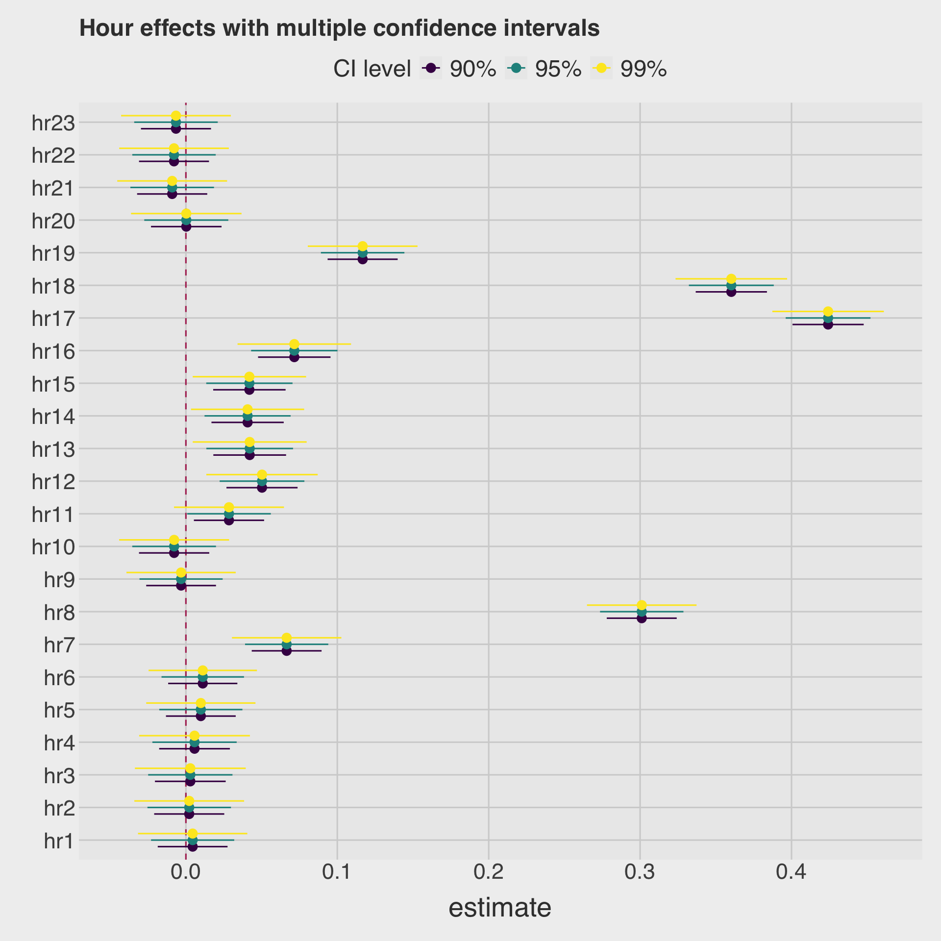
- Draw a coefficient plot for
hrvariables.
Show answer
model_betas <- tidy(model,
conf.int = T) # conf.level = 0.95 (default)
model_betas_90ci <- tidy(model,
conf.int = T,
conf.level = 0.90)
model_betas_99ci <- tidy(model,
conf.int = T,
conf.level = 0.99)
# Add a CI label to each and row-bind
month_ci <- bind_rows(
model_betas_90ci |> mutate(ci = "90%"),
model_betas |> mutate(ci = "95%"),
model_betas_99ci |> mutate(ci = "99%")
) |>
filter(str_detect(term, "hr")) |>
mutate(term = factor(term,
levels = str_c("hr", 1:23))
)|>
mutate(ci = factor(ci, levels = c("90%", "95%", "99%")))
ggplot(
month_ci,
aes(
y = term,
x = estimate,
xmin = conf.low,
xmax = conf.high,
color = ci
)
) +
geom_vline(xintercept = 0, color = "maroon", linetype = 2) +
geom_pointrange(
position = position_dodge(width = 0.6)
) +
labs(
title = "Hour effects with multiple confidence intervals",
color = "CI level",
y = ""
) 
Q1d
- Using the estimation result in Q1a:
- Make a prediction on the outcome variable using the test data.frame.
Show answer
model_pred_test <- augment(model, newdata = dtest)
rmarkdown::paged_table(model_pred_test)Q1e
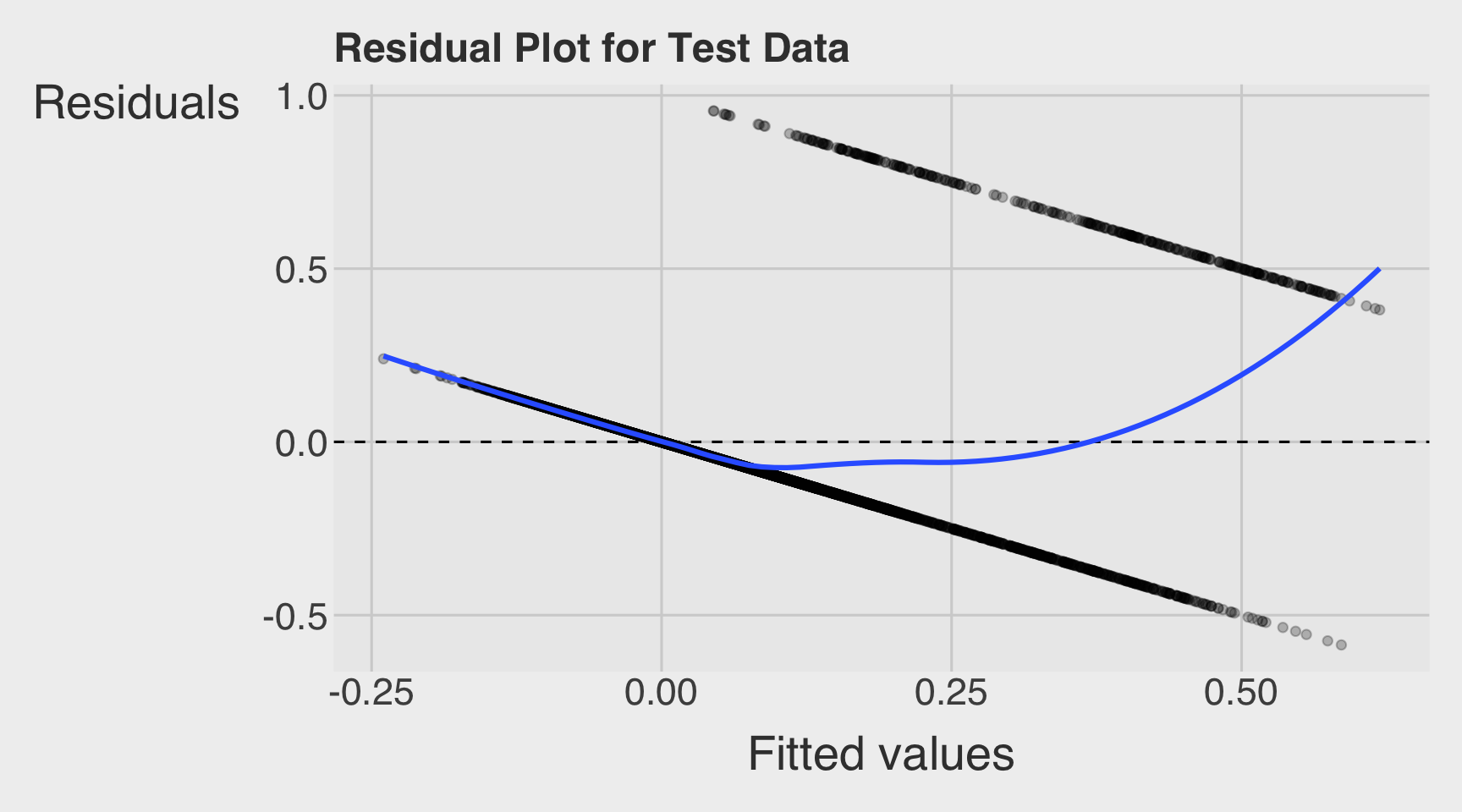
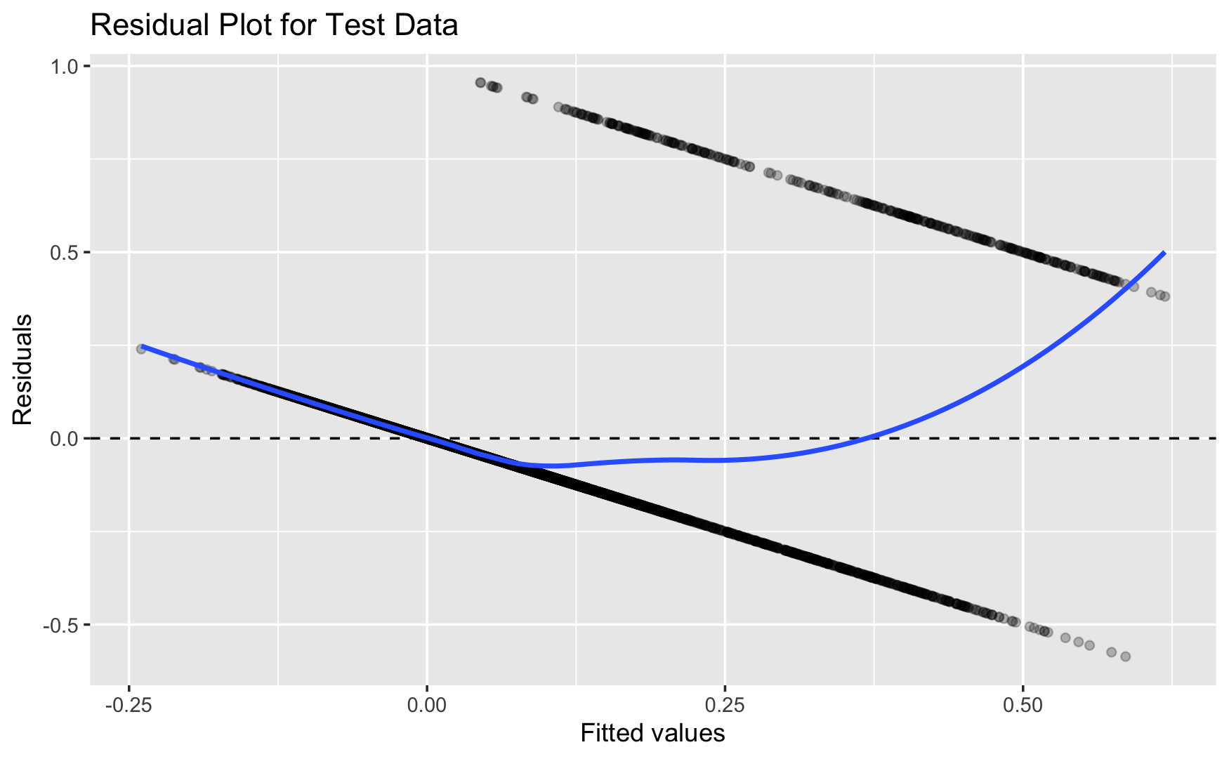
- Draw a residual plot using the test data.frame.
Show answer
model_pred_test |>
mutate(.resid = over_load - .fitted) |>
ggplot(aes(x = .fitted, y = .resid)) +
geom_point(alpha = 0.25) +
geom_hline(yintercept = 0, linetype = "dashed") +
geom_smooth(se = FALSE, method = "loess") +
labs(
x = "Fitted values",
y = "Residuals",
title = "Residual Plot for Test Data"
)
Section 2. Logistic Regression
Q2a
Use R to fit the following logistic regression model:
\[ \begin{align} \text{Prob}(\text{over\_load}_{i} = 1) =\ G(\;\; &\beta_{\text{intercept}}\\ &+ \beta_{\text{temp}} \, \text{temp}_{i} + \beta_{\text{hum}} \, \text{hum}_{i} + \beta_{\text{windspeed}} \, \text{windspeed}_{i} \nonumber \\ &+ \beta_{\text{year\_2012}} \, \text{year\_2012}_{i}\\ &+ \beta_{\text{month\_2}} \, \text{month\_2}_{i} + \beta_{\text{month\_3}} \, \text{month\_3}_{i} + \beta_{\text{month\_4}} \, \text{month\_4}_{i} \nonumber \\ &+ \beta_{\text{month\_5}} \, \text{month\_5}_{i} + \beta_{\text{month\_6}} \, \text{month\_6}_{i} + \beta_{\text{month\_7}} \, \text{month\_7}_{i} \nonumber \\ &+ \beta_{\text{month\_8}} \, \text{month\_8}_{i} + \beta_{\text{month\_9}} \, \text{month\_9}_{i} + \beta_{\text{month\_10}} \, \text{month\_10}_{i} \nonumber \\ &+ \beta_{\text{month\_11}} \, \text{month\_11}_{i} + \beta_{\text{month\_12}} \, \text{month\_12}_{i} \nonumber \\ &+ \beta_{\text{hr\_1}} \, \text{hr\_1}_{i} + \beta_{\text{hr\_2}} \, \text{hr\_2}_{i} + \beta_{\text{hr\_3}} \, \text{hr\_3}_{i} + \beta_{\text{hr\_4}} \, \text{hr\_4}_{i} \nonumber \\ &+ \beta_{\text{hr\_5}} \, \text{hr\_5}_{i} + \beta_{\text{hr\_6}} \, \text{hr\_6}_{i} + \beta_{\text{hr\_7}} \, \text{hr\_7}_{i} + \beta_{\text{hr\_8}} \, \text{hr\_8}_{i} \nonumber \\ &+ \beta_{\text{hr\_9}} \, \text{hr\_9}_{i} + \beta_{\text{hr\_10}} \, \text{hr\_10}_{i} + \beta_{\text{hr\_11}} \, \text{hr\_11}_{i} + \beta_{\text{hr\_12}} \, \text{hr\_12}_{i} \nonumber \\ &+ \beta_{\text{hr\_13}} \, \text{hr\_13}_{i} + \beta_{\text{hr\_14}} \, \text{hr\_14}_{i} + \beta_{\text{hr\_15}} \, \text{hr\_15}_{i} + \beta_{\text{hr\_16}} \, \text{hr\_16}_{i} \nonumber \\ &+ \beta_{\text{hr\_17}} \, \text{hr\_17}_{i} + \beta_{\text{hr\_18}} \, \text{hr\_18}_{i} + \beta_{\text{hr\_19}} \, \text{hr\_19}_{i} + \beta_{\text{hr\_20}} \, \text{hr\_20}_{i} \nonumber \\ &+ \beta_{\text{hr\_21}} \, \text{hr\_21}_{i} + \beta_{\text{hr\_22}} \, \text{hr\_22}_{i} + \beta_{\text{hr\_23}} \, \text{hr\_23}_{i} \nonumber \\ &+ \beta_{\text{wkday\_monday}} \, \text{wkday\_monday}_{i} + \beta_{\text{wkday\_tuesday}} \, \text{wkday\_tuesday}_{i} \nonumber \\ &+ \beta_{\text{wkday\_wednesday}} \, \text{wkday\_wednesday}_{i} \nonumber \\ &+ \beta_{\text{wkday\_thursday}} \, \text{wkday\_thursday}_{i} + \beta_{\text{wkday\_friday}} \, \text{wkday\_friday}_{i} \nonumber \\ &+ \beta_{\text{wkday\_saturday}} \, \text{wkday\_saturday}_{i} \nonumber \\ &+ \beta_{\text{holiday\_1}} \, \text{holiday\_1}_{i} \nonumber \\ &+ \beta_{\text{seasons\_summer}} \, \text{seasons\_summer}_{i} + \beta_{\text{seasons\_fall}} \, \text{seasons\_fall}_{i} \nonumber \\ &+ \beta_{\text{seasons\_winter}} \, \text{seasons\_winter}_{i} \nonumber \\ &+ \beta_{\text{weather\_cond\_Light\_Snow\_or\_Light\_Rain}} \, \text{weather\_cond\_Light\_Snow\_or\_Light\_Rain}_{i}\nonumber \\ &+ \beta_{\text{weather\_cond\_Mist\_or\_Cloudy}} \, \text{weather\_cond\_Mist\_or\_Cloudy}_{i} \;\;) \end{align} \]
where \(G(\,\cdot\,)\) is
\[ G(\,\cdot\,) = \frac{\exp(\,\cdot\,)}{1 + \exp(\,\cdot\,)}. \]
- Provide a table that summarize the estimation result, including beta estimates, AIC, and residual deviance.
Show answer
model_logit <- glm(
over_load ~ temp + hum + windspeed +
year +
month +
hr +
wkday +
holiday +
seasons +
weather_cond,
data = dtrain,
family = binomial(link = "logit")
)Q2b
- Using the estimation result in Q2a:
- Calculate the average marginal effect of
hrandwkdaydummies.
- Calculate the average marginal effect of
Show answer
summary(
margins(model_logit,
variables = c("hr", "wkday"))
) factor AME SE z p lower upper
hr1 0.0000 0.0000 0.0000 1.0000 -0.0000 0.0000
hr10 0.0020 0.0020 1.0051 0.3148 -0.0019 0.0060
hr11 0.0414 0.0077 5.3733 0.0000 0.0263 0.0565
hr12 0.0620 0.0093 6.6507 0.0000 0.0437 0.0803
hr13 0.0545 0.0087 6.2328 0.0000 0.0373 0.0716
hr14 0.0546 0.0087 6.2593 0.0000 0.0375 0.0717
hr15 0.0533 0.0086 6.2012 0.0000 0.0364 0.0701
hr16 0.0777 0.0102 7.5896 0.0000 0.0576 0.0978
hr17 0.4169 0.0173 24.0827 0.0000 0.3829 0.4508
hr18 0.3430 0.0163 21.0405 0.0000 0.3110 0.3749
hr19 0.1171 0.0117 10.0411 0.0000 0.0943 0.1400
hr2 0.0000 0.0000 0.0000 1.0000 -0.0000 0.0000
hr20 0.0133 0.0049 2.7255 0.0064 0.0037 0.0229
hr21 0.0021 0.0021 1.0051 0.3148 -0.0020 0.0062
hr22 -0.0000 0.0000 -0.0002 0.9999 -0.0000 0.0000
hr23 -0.0000 0.0000 -0.0001 0.9999 -0.0000 0.0000
hr3 0.0000 0.0000 0.0001 0.9999 -0.0000 0.0000
hr4 0.0000 0.0000 0.0001 0.9999 -0.0000 0.0000
hr5 0.0000 0.0000 0.0002 0.9998 -0.0000 0.0000
hr6 0.0000 0.0000 0.0002 0.9998 -0.0000 0.0000
hr7 0.0813 0.0130 6.2380 0.0000 0.0557 0.1068
hr8 0.3348 0.0164 20.4017 0.0000 0.3026 0.3669
hr9 -0.0000 0.0000 -0.0001 1.0000 -0.0000 0.0000
wkdayfriday -0.0010 0.0061 -0.1722 0.8633 -0.0130 0.0109
wkdaymonday 0.0143 0.0066 2.1571 0.0310 0.0013 0.0272
wkdaysaturday 0.0156 0.0063 2.4637 0.0137 0.0032 0.0280
wkdaythursday 0.0113 0.0062 1.8368 0.0662 -0.0008 0.0234
wkdaytuesday 0.0234 0.0064 3.6539 0.0003 0.0108 0.0359
wkdaywednesday 0.0184 0.0064 2.8985 0.0037 0.0060 0.0309Q2c
- Using the estimation result in Q2a:
- Make a prediction on training data
- Make a prediction on test data
Show answer
model_logit_pred_train <- model_logit |>
augment(type.predict = "response")
model_logit_pred_test <- model_logit |>
augment(type.predict = "response",
newdata = dtest)
model_logit_pred_train |>
paged_table()model_logit_pred_test |>
paged_table()Q2d
- Using the estimation result in Q2a:
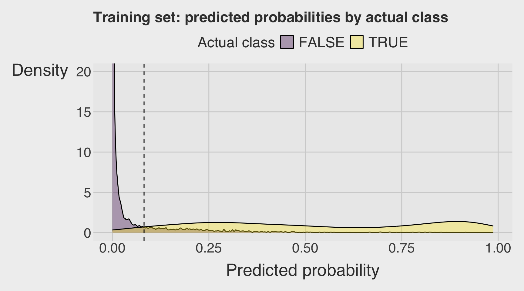
- Visualize a double density plot of predictions from the training data.
coord_cartesian(ylim = c(0, 20))can help identify the threshold.
- Visualize a double density plot of predictions from the training data.
Show answer
threshold <- 0.082
model_logit_pred_train |>
ggplot(aes(x = .fitted,
fill = factor(over_load))) +
geom_density(alpha = 0.35) +
geom_vline(xintercept = threshold, linetype = "dashed") +
coord_cartesian(ylim = c(0, 20)) +
labs(
x = "Predicted probability",
y = "Density",
fill = "Actual class",
title = "Training set: predicted probabilities by actual class"
)
Q2e
- Using the estimation result in Q2a, calculate the followings:
- Confusion matrix with the threshold level that clearly separates the double density plots
- Accuracy
- Precision
- Recall
- Specificity
- Base rate
- Enrichment
Show answer
Confusion Matrix
# threshold <- mean(dtest$over_load)
df_cm <- model_logit_pred_test |>
mutate(
over_load = as.integer(over_load),
actual = factor(over_load,
levels = c(0, 1),
labels = c("not overloaded", "overloaded")),
pred = factor(ifelse(.fitted > threshold, 1, 0),
levels = c(0, 1),
labels = c("not overloaded", "overloaded"))
)
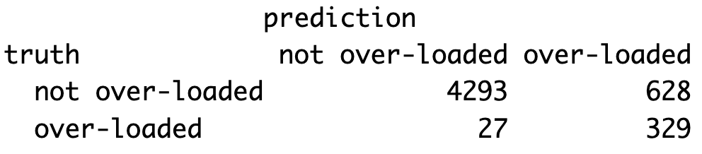
conf_mat <- table(truth = df_cm$actual,
prediction = df_cm$pred)
conf_mat prediction
truth not overloaded overloaded
not overloaded 4293 628
overloaded 27 329Performance Metrics
base_rate <- mean(dtest$over_load)
accuracy <- (conf_mat[1,1] + conf_mat[2,2]) / sum(conf_mat)
precision <- conf_mat[2,2] / sum(conf_mat[,2])
recall <- conf_mat[2,2] / sum(conf_mat[2,])
specificity <- conf_mat[1,1] / sum(conf_mat[1,])
enrichment <- precision / base_rate
df_class_metric <-
data.frame(
metric = c("Base rate",
"Accuracy",
"Precision",
"Recall",
"Specificity",
"Enrichment"),
value = c(base_rate,
accuracy,
precision,
recall,
specificity,
enrichment)
)
df_class_metric |>
mutate(value = round(value, 4)) |>
rmarkdown::paged_table()Q2f
- Using the estimation result in Q2a
- Visualize the variation in recall and enrichment across different threshold levels.
Show answer
plt <- PRTPlot(df_cm,
".fitted", "over_load", 1,
plotvars = c("enrichment", "recall"),
thresholdrange = c(0,.1),
title = "Enrichment vs. recall with threshold")
plt +
geom_vline(xintercept = threshold,
color="maroon",
linetype = 2)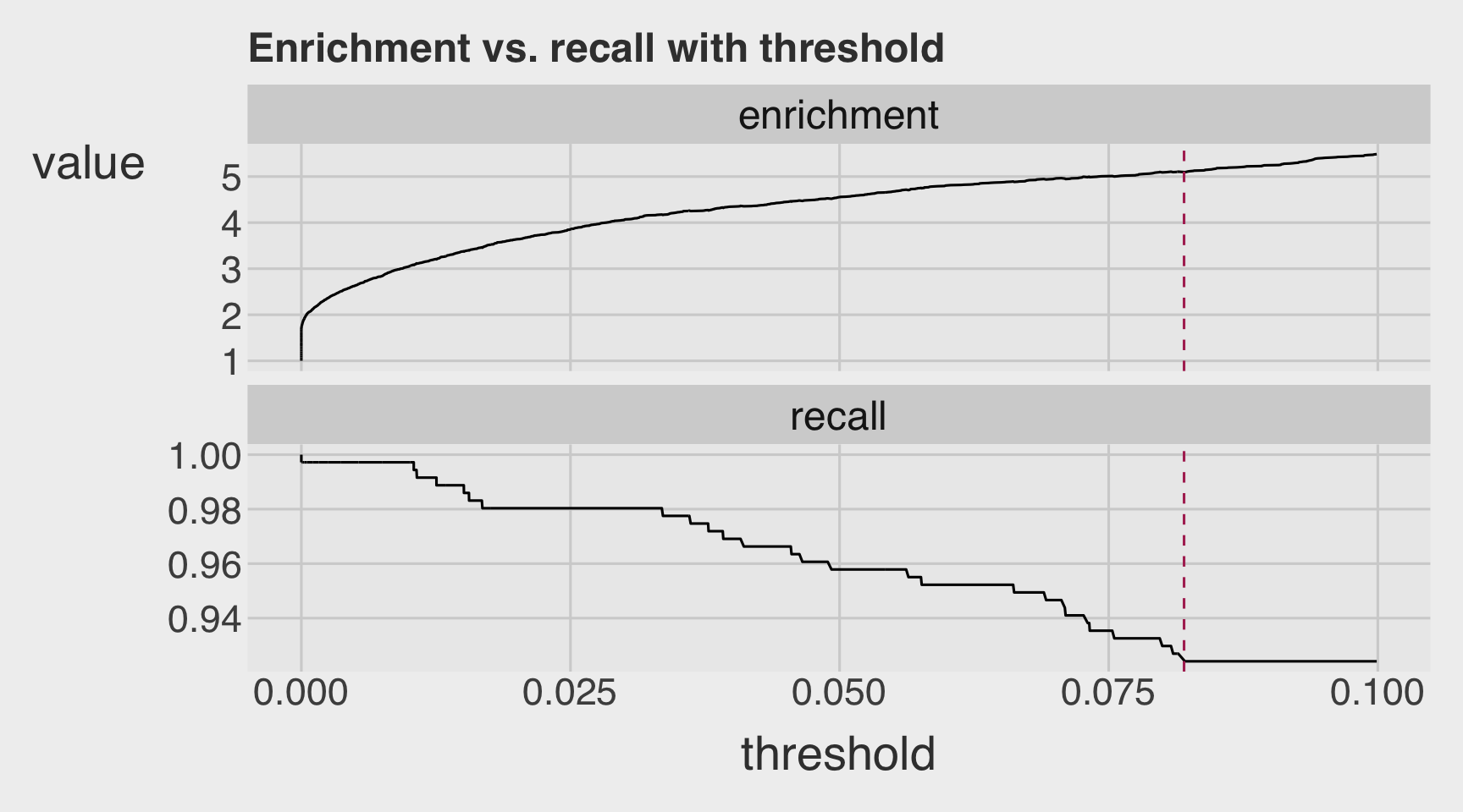
Q2g
- Using the estimation result in Q2a
- Draw the receiver operating characteristic (ROC) curve.
- Calculate the area under the curve (AUC).
Show answer
roc <- ROCPlot(df_cm,
xvar = '.fitted',
truthVar = 'over_load',
truthTarget = 1,
title = 'Classifier performance')
# ROC with vertical line
roc +
geom_vline(xintercept = 1 - specificity,
color="maroon", linetype = 2)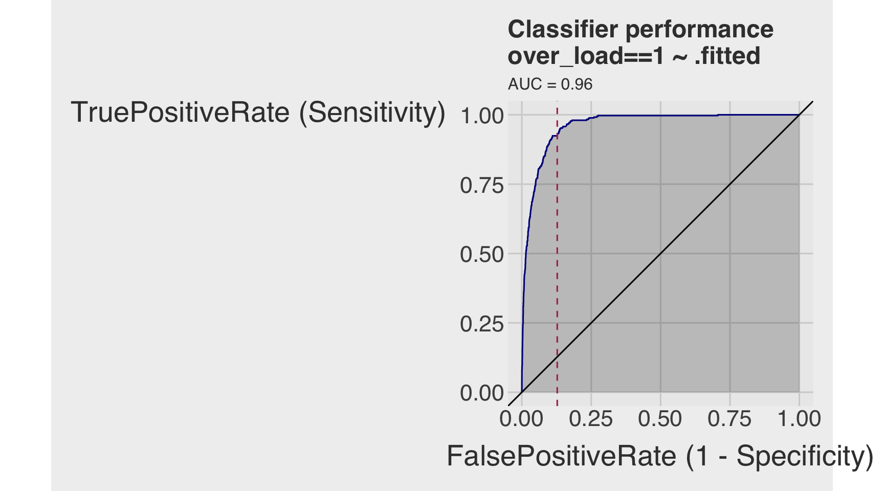
# AUC
# pROC::roc(BINARY_OUTCOME, PREDICTED_PROBABILITY)
roc_obj <- roc(df_cm$over_load, df_cm$.fitted)
auc(roc_obj)Area under the curve: 0.9621Section 3. Regularized Regression
Q3a
Prepare the data for regularized regression.
Tasks 1–2
Using the dtrain and dtest data.frames, complete the following:
- Convert the logical response variable
over_loadto an integer vector:- Create
y_trainfromover_loadindtrain - Create
y_testfromover_loadindtest
- Create
- Construct predictor matrices:
- Create
X_trainusing all continuous and dummy predictors indtrain - Create
X_testusing all continuous and dummy predictors indtest
- Create
Show answer
# y must be numeric 0/1 (FALSE->0, TRUE->1)
y_train <- as.integer(dtrain$over_load)
y_test <- as.integer(dtest$over_load)
# x must be a numeric matrix
# [, -1] to remove an intercept variable
X_train <- model.matrix(~ temp + hum + windspeed +
year +
month +
hr +
wkday +
holiday +
seasons +
weather_cond, data = dtrain)[, -1]
X_test <- model.matrix(~ temp + hum + windspeed +
year +
month +
hr +
wkday +
holiday +
seasons +
weather_cond, data = dtest)[, -1]Data for Regularization: y_train, y_test, X_train, and X_test
If you were not able to successfully prepare the data for regularized model estimation, you may use the training (y_train and X_train) and test (y_test and X_test) data provided in Section 0.
Q3b
- Fit a 7-fold cross-validated (CV) Lasso logistic regression, providing
- Beta estimates
- Optimal lambdas
- Plot for CV curve
- Plot for coefficient path
- Plot for the number of nonzero betas as a function of a lambda
- Classification performance, including accuracy, precision, recall, and AUC.
Show answer
Fitting CV Lasso
set.seed(1)
model_lasso <- cv.glmnet(
X_train, y_train,
alpha = 1,
nfolds = 7, # 10 is default
family = "binomial"
)Betas
# Lasso
beta_lasso_1se <- coef(model_lasso,
s = "lambda.1se") # default
beta_lasso_min <- coef(model_lasso,
s = "lambda.min")
betas <- data.frame(
term = rownames(beta_lasso_1se),
beta_lasso_1se = as.numeric(beta_lasso_1se),
beta_lasso_min = as.numeric(beta_lasso_min)
)
# Show only nonzero in either solution
betas_lasso_nz <- betas |>
filter(beta_lasso_1se != 0 | beta_lasso_min != 0) |>
arrange(abs(beta_lasso_1se), abs(beta_lasso_min))
betas |>
paged_table(options =
list(
rows.print = nrow(betas)
)
)Optimal Lambdas
lambdas_lasso <- model_lasso |>
glance()
lambdas_lasso |>
paged_table()CV Curve
# Run all at once
par(mar = c(5.1, 4.1, 6.1, 2.1)) # title margin
plot(model_lasso, main = "Lasso")
abline(v = log(model_lasso$lambda.min), lty = 2)
abline(v = log(model_lasso$lambda.1se), lty = 3)
legend("bottomright",
legend = c("lambda.min", "lambda.1se"),
lty = c(2, 3),
bty = "n")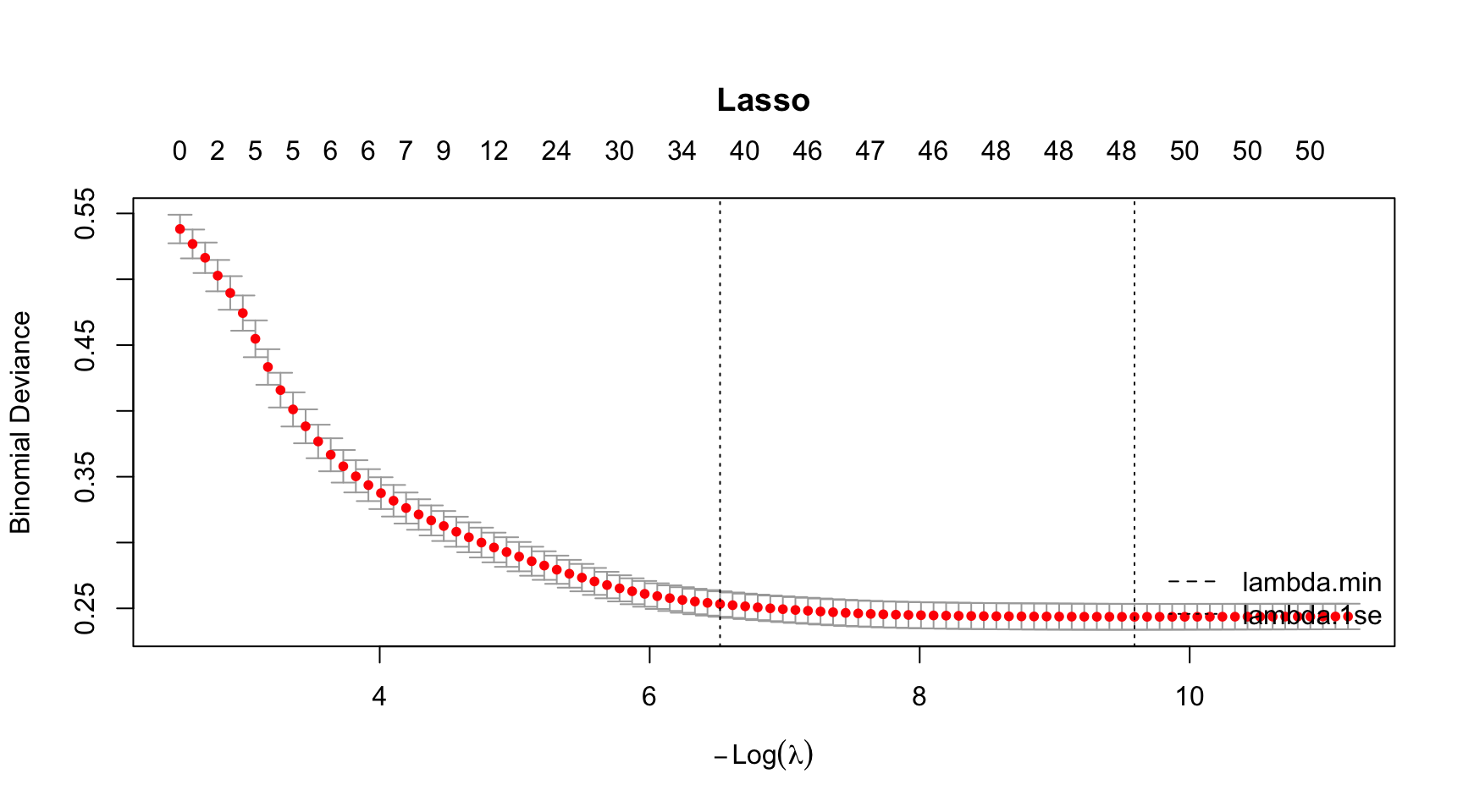
Lasso Coefficient Path
# Run all at once
par(mar = c(5.1, 4.1, 6.1, 2.1)) # title margin
plot(model_lasso$glmnet.fit, xvar = "lambda",
main = "Lasso")
abline(v = log(model_lasso$lambda.min), lty = 2)
abline(v = log(model_lasso$lambda.1se), lty = 3)
legend("topright",
legend = c("lambda.min", "lambda.1se"),
lty = c(2, 3),
bty = "n")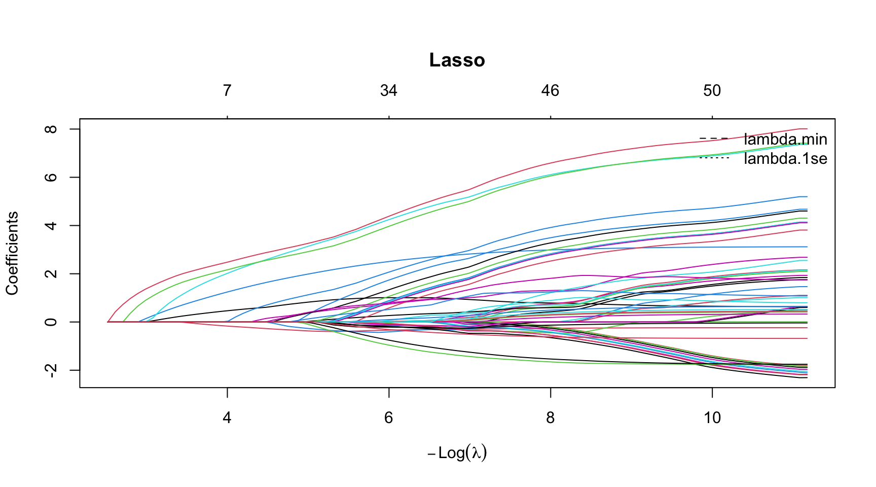
Number of Non-zero betas as a function of a lambda
CVErrors_lasso <- tidy(model_lasso)
CVErrors_lasso |>
ggplot(aes(x = lambda,
y = nzero)) +
geom_point() +
geom_line()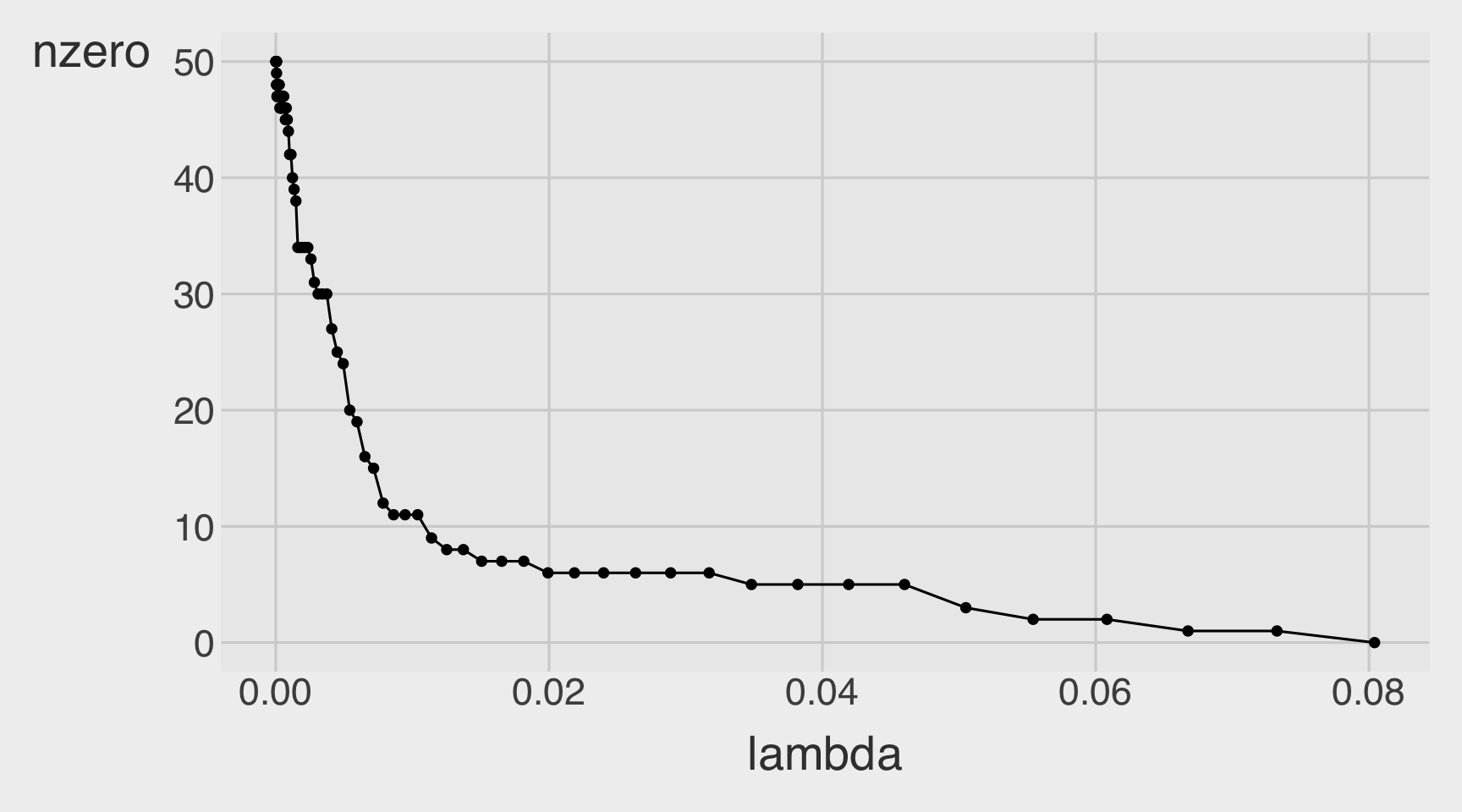
Classification performance, including accuracy, precision, recall, and AUC.
Prediction
# threshold <- mean(dtest$over_load)
df_cm_all_lasso <- dtest |>
mutate(
.fitted_lasso_1se = predict(model_lasso, newx = X_test,
s = "lambda.1se", type = "response"),
.fitted_lasso_min = predict(model_lasso, newx = X_test,
s = "lambda.min", type = "response")
) |>
mutate(
over_load = as.integer(over_load),
actual = factor(over_load,
levels = c(0, 1),
labels = c("not overloaded", "overloaded")),
pred_lasso_1se = factor(ifelse(.fitted_lasso_1se > threshold, 1, 0),
levels = c(0, 1),
labels = c("not overloaded", "overloaded")),
pred_lasso_min = factor(ifelse(.fitted_lasso_min > threshold, 1, 0),
levels = c(0, 1),
labels = c("not overloaded", "overloaded"))
)Confusion Matrices
# Lasso Logistic 1se
conf_mat_lasso_1se <- table(truth = df_cm_all_lasso$actual,
prediction_lasso_1se = df_cm_all_lasso$pred_lasso_1se)
conf_mat_lasso_1se prediction_lasso_1se
truth not overloaded overloaded
not overloaded 4274 647
overloaded 22 334# Lasso Logistic min
conf_mat_lasso_min <- table(truth = df_cm_all_lasso$actual,
prediction_lasso_min = df_cm_all_lasso$pred_lasso_min)
conf_mat_lasso_min prediction_lasso_min
truth not overloaded overloaded
not overloaded 4292 629
overloaded 25 331Performance Metrics
base_rate <- mean(dtest$over_load)
# Lasso Logistic 1se
accuracy_lasso_1se <- (conf_mat_lasso_1se[1,1] + conf_mat_lasso_1se[2,2]) / sum(conf_mat_lasso_1se)
precision_lasso_1se <- conf_mat_lasso_1se[2,2] / sum(conf_mat_lasso_1se[,2])
recall_lasso_1se <- conf_mat_lasso_1se[2,2] / sum(conf_mat_lasso_1se[2,])
specificity_lasso_1se <- conf_mat_lasso_1se[1,1] / sum(conf_mat_lasso_1se[1,])
enrichment_lasso_1se <- precision_lasso_1se / base_rate
# Lasso Logistic min
accuracy_lasso_min <- (conf_mat_lasso_min[1,1] + conf_mat_lasso_min[2,2]) / sum(conf_mat_lasso_min)
precision_lasso_min <- conf_mat_lasso_min[2,2] / sum(conf_mat_lasso_min[,2])
recall_lasso_min <- conf_mat_lasso_min[2,2] / sum(conf_mat_lasso_min[2,])
specificity_lasso_min <- conf_mat_lasso_min[1,1] / sum(conf_mat_lasso_min[1,])
enrichment_lasso_min <- precision_lasso_min / base_rate
df_class_metric_lasso <-
data.frame(
metric = c("Base rate",
"Accuracy",
"Precision",
"Recall",
"Specificity",
"Enrichment"),
value_lasso_1se = c(base_rate,
accuracy_lasso_1se,
precision_lasso_1se,
recall_lasso_1se,
specificity_lasso_1se,
enrichment_lasso_1se),
value_lasso_min = c(base_rate,
accuracy_lasso_min,
precision_lasso_min,
recall_lasso_min,
specificity_lasso_min,
enrichment_lasso_min)
)
df_class_metric_lasso |>
mutate(value_lasso_1se = round(value_lasso_1se, 4),
value_lasso_min = round(value_lasso_min, 4),
) |>
rmarkdown::paged_table()AUC
roc_lasso_1se <- ROCPlot(df_cm_all_lasso,
xvar = '.fitted_lasso_1se',
truthVar = 'over_load',
truthTarget = 1,
title = 'Classifier performance')
# ROC with vertical line
roc_lasso_1se +
geom_vline(xintercept = 1 - specificity_lasso_1se,
color="maroon", linetype = 2)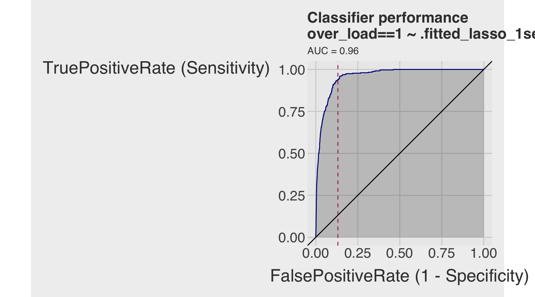
roc_obj_lasso_1se <- roc(df_cm_all_lasso$over_load, df_cm_all_lasso$.fitted_lasso_1se)
auc(roc_obj_lasso_1se)Area under the curve: 0.9593Q3c
- Fit a 7-fold cross-validated (CV) Ridge logistic regression, providing
- Beta estimates
- Optimal lambdas
- Plot for CV curve
- Plot for coefficient path
- Plot for the number of nonzero betas as a function of a lambda
- Classification performance, including accuracy, precision, recall, and AUC.
Show answer
Fitting CV ridge
set.seed(1)
model_ridge <- cv.glmnet(
X_train, y_train,
alpha = 0,
nfolds = 7, # 10 is default
family = "binomial"
)Betas
# ridge
beta_ridge_1se <- coef(model_ridge,
s = "lambda.1se") # default
beta_ridge_min <- coef(model_ridge,
s = "lambda.min")
betas <- data.frame(
term = rownames(beta_ridge_1se),
beta_ridge_1se = as.numeric(beta_ridge_1se),
beta_ridge_min = as.numeric(beta_ridge_min)
)
# Show only nonzero in either solution
betas_ridge_nz <- betas |>
filter(beta_ridge_1se != 0 | beta_ridge_min != 0) |>
arrange(abs(beta_ridge_1se), abs(beta_ridge_min))
betas |>
paged_table(options =
list(
rows.print = nrow(betas)
)
)Optimal Lambdas
lambdas_ridge <- model_ridge |>
glance()
lambdas_ridge |>
paged_table()CV Curve
# Run all at once
par(mar = c(5.1, 4.1, 6.1, 2.1)) # title margin
plot(model_ridge, main = "ridge")
abline(v = log(model_ridge$lambda.min), lty = 2)
abline(v = log(model_ridge$lambda.1se), lty = 3)
legend("bottomright",
legend = c("lambda.min", "lambda.1se"),
lty = c(2, 3),
bty = "n")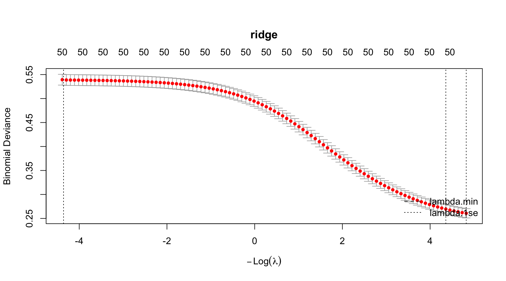
ridge Coefficient Path
# Run all at once
par(mar = c(5.1, 4.1, 6.1, 2.1)) # title margin
plot(model_ridge$glmnet.fit, xvar = "lambda",
main = "ridge")
abline(v = log(model_ridge$lambda.min), lty = 2)
abline(v = log(model_ridge$lambda.1se), lty = 3)
legend("topright",
legend = c("lambda.min", "lambda.1se"),
lty = c(2, 3),
bty = "n")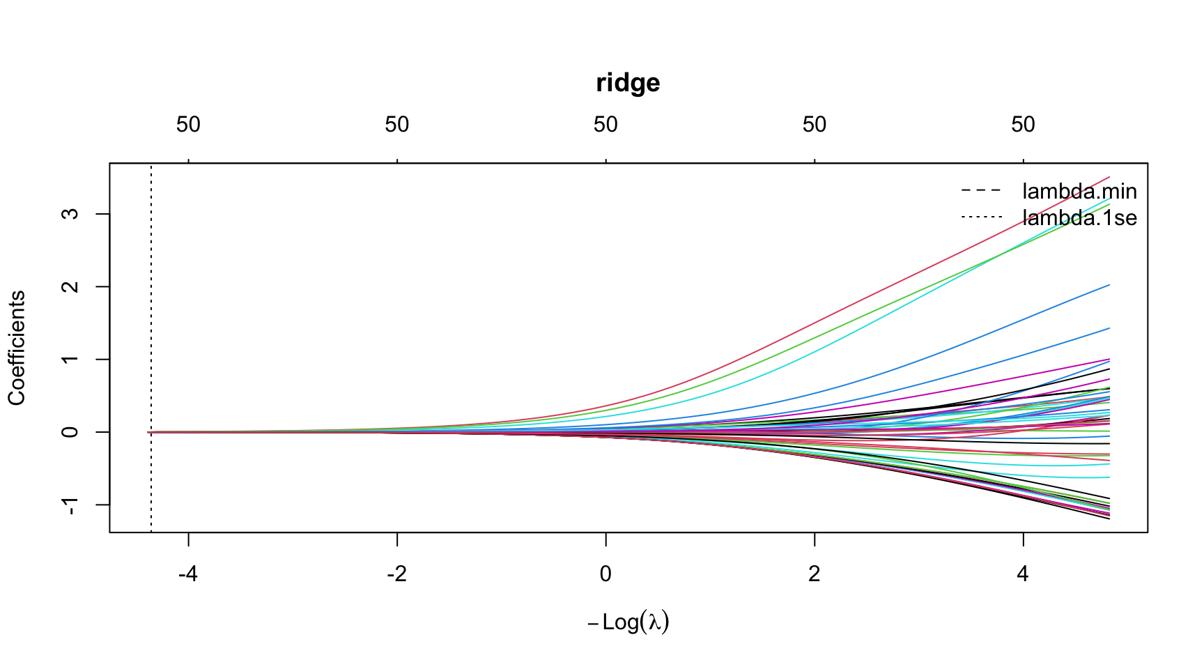
Number of Non-zero betas as a function of a lambda
CVErrors_ridge <- tidy(model_ridge)
CVErrors_ridge |>
ggplot(aes(x = lambda,
y = nzero)) +
geom_point() +
geom_line()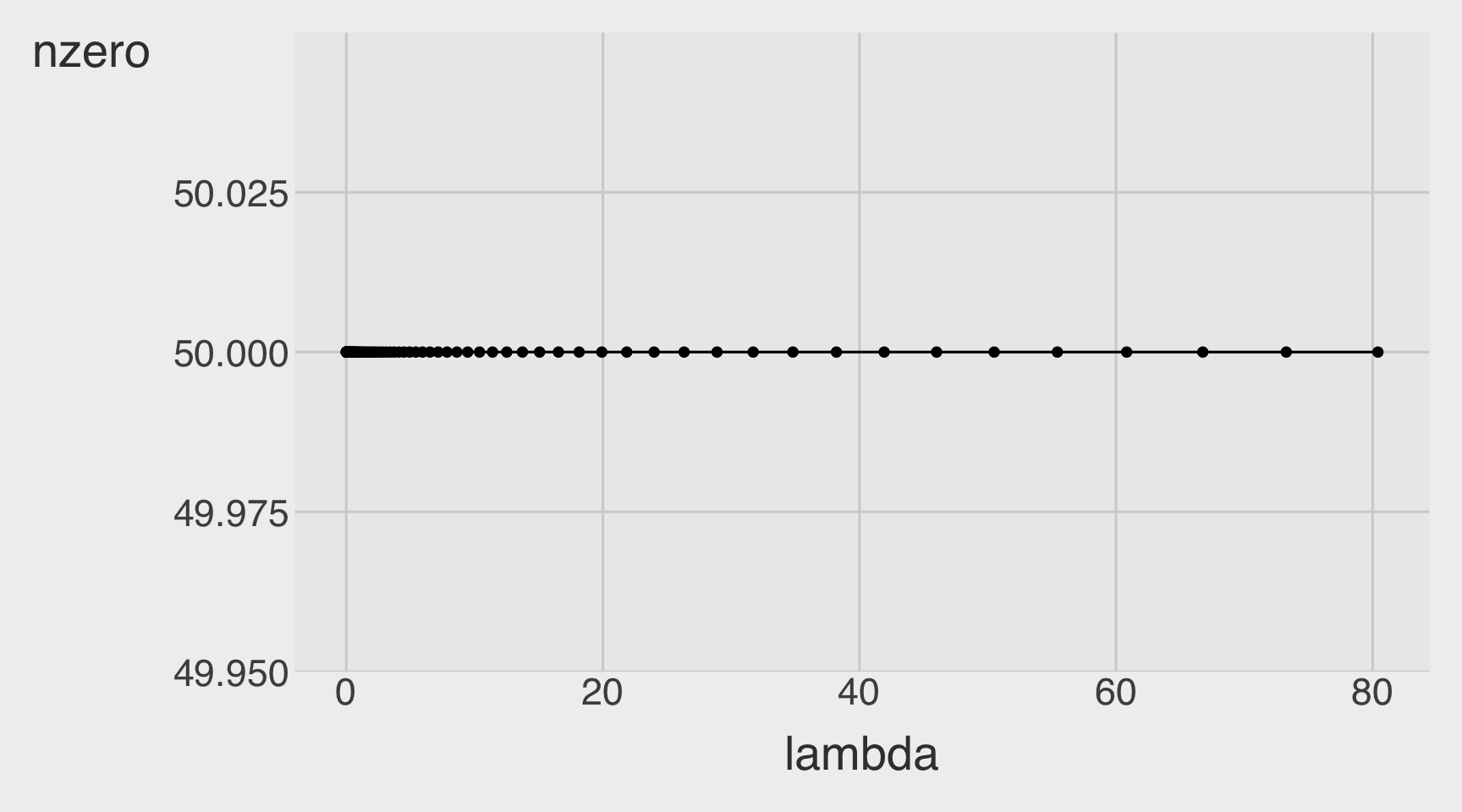
Classification performance, including accuracy, precision, recall, and AUC.
Prediction
# threshold <- mean(dtest$over_load)
df_cm_all_ridge <- dtest |>
mutate(
.fitted_ridge_1se = predict(model_ridge, newx = X_test,
s = "lambda.1se", type = "response"),
.fitted_ridge_min = predict(model_ridge, newx = X_test,
s = "lambda.min", type = "response")
) |>
mutate(
over_load = as.integer(over_load),
actual = factor(over_load,
levels = c(0, 1),
labels = c("not overloaded", "overloaded")),
pred_ridge_1se = factor(ifelse(.fitted_ridge_1se > threshold, 1, 0),
levels = c(0, 1),
labels = c("not overloaded", "overloaded")),
pred_ridge_min = factor(ifelse(.fitted_ridge_min > threshold, 1, 0),
levels = c(0, 1),
labels = c("not overloaded", "overloaded"))
)Confusion Matrices
# ridge Logistic 1se
conf_mat_ridge_1se <- table(truth = df_cm_all_ridge$actual,
prediction_ridge_1se = df_cm_all_ridge$pred_ridge_1se)
conf_mat_ridge_1se prediction_ridge_1se
truth not overloaded overloaded
not overloaded 4164 757
overloaded 18 338# ridge Logistic min
conf_mat_ridge_min <- table(truth = df_cm_all_ridge$actual,
prediction_ridge_min = df_cm_all_ridge$pred_ridge_min)
conf_mat_ridge_min prediction_ridge_min
truth not overloaded overloaded
not overloaded 4196 725
overloaded 17 339Performance Metrics
base_rate <- mean(dtest$over_load)
# ridge Logistic 1se
accuracy_ridge_1se <- (conf_mat_ridge_1se[1,1] + conf_mat_ridge_1se[2,2]) / sum(conf_mat_ridge_1se)
precision_ridge_1se <- conf_mat_ridge_1se[2,2] / sum(conf_mat_ridge_1se[,2])
recall_ridge_1se <- conf_mat_ridge_1se[2,2] / sum(conf_mat_ridge_1se[2,])
specificity_ridge_1se <- conf_mat_ridge_1se[1,1] / sum(conf_mat_ridge_1se[1,])
enrichment_ridge_1se <- precision_ridge_1se / base_rate
# ridge Logistic min
accuracy_ridge_min <- (conf_mat_ridge_min[1,1] + conf_mat_ridge_min[2,2]) / sum(conf_mat_ridge_min)
precision_ridge_min <- conf_mat_ridge_min[2,2] / sum(conf_mat_ridge_min[,2])
recall_ridge_min <- conf_mat_ridge_min[2,2] / sum(conf_mat_ridge_min[2,])
specificity_ridge_min <- conf_mat_ridge_min[1,1] / sum(conf_mat_ridge_min[1,])
enrichment_ridge_min <- precision_ridge_min / base_rate
df_class_metric_ridge <-
data.frame(
metric = c("Base rate",
"Accuracy",
"Precision",
"Recall",
"Specificity",
"Enrichment"),
value_ridge_1se = c(base_rate,
accuracy_ridge_1se,
precision_ridge_1se,
recall_ridge_1se,
specificity_ridge_1se,
enrichment_ridge_1se),
value_ridge_min = c(base_rate,
accuracy_ridge_min,
precision_ridge_min,
recall_ridge_min,
specificity_ridge_min,
enrichment_ridge_min)
)
df_class_metric_ridge |>
mutate(value_ridge_1se = round(value_ridge_1se, 4),
value_ridge_min = round(value_ridge_min, 4),
) |>
rmarkdown::paged_table()AUC
roc_ridge_1se <- ROCPlot(df_cm_all_ridge,
xvar = '.fitted_ridge_1se',
truthVar = 'over_load',
truthTarget = 1,
title = 'Classifier performance')
# ROC with vertical line
roc_ridge_1se +
geom_vline(xintercept = 1 - specificity_ridge_1se,
color="maroon", linetype = 2)
roc_obj_ridge_1se <- roc(df_cm_all_ridge$over_load, df_cm_all_ridge$.fitted_ridge_1se)
auc(roc_obj_ridge_1se)Area under the curve: 0.9567Classification Performances Across All Models
df_class_metric_all <- df_class_metric |>
left_join(df_class_metric_lasso) |>
left_join(df_class_metric_ridge)
df_class_metric_all |>
paged_table()Section 4. Understanding ML Models
Q4a. Residual Plots
Below is the residual plot from the linear regression model fit from Q1a in Section 1:
What is the meaning of the fitted value from the linear regression model in Section 1?
On average, are the predictions correct in the linear regression model in Q1a?
Are there systematic errors?
Show answer
The fitted value from the linear regression model is the model’s predicted value of the response variable for a given observation, based on its predictor values.
- In this case, because the response variable is binary, the fitted value can be interpreted as the model’s predicted probability that the outcome equals \(1\).
On average, the predictions are approximately correct if the residuals are centered around \(0\). In the plot, the smooth line stays fairly close to \(0\) in the middle range, so the model is not badly biased overall.
Yes, there appear to be systematic errors.
- The residual smooth curve is not flat and instead shows a curved pattern, suggesting nonlinearity or model misspecification. This means the linear regression model tends to overpredict in some fitted-value ranges.
- Additionally, instead of forming a random cloud around the perfect-prediction line at residual \(= 0\), the points fall along two straight diagonal lines. This happens because the outcome is binary: each observed response is either \(0\) or \(1\), and the residual is computed as \(y - \hat{y}\). So when \(y = 0\), the residuals lie on the line \(-\hat{y}\), and when \(y = 1\), the residuals lie on the line \(1 - \hat{y}\). This striped pattern is typical when using linear regression for a binary outcome.
- Some fitted values are also negative, which implies negative predicted probabilities. Since probabilities should lie between \(0\) and \(1\), this is another sign that the linear regression model may not be appropriate for predicting a binary outcome.
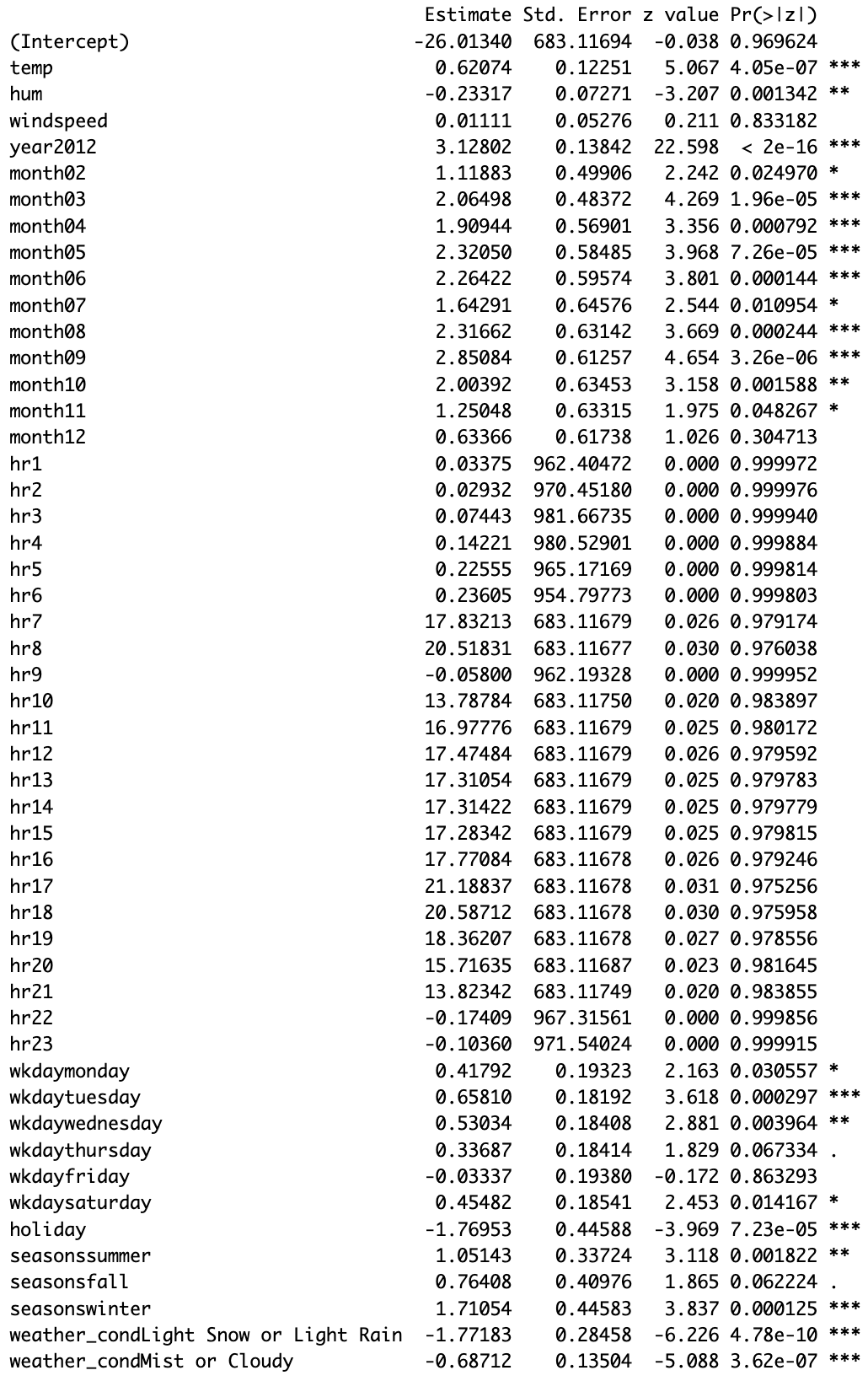
Q4b. Beta Estimates in Logistic regression
Below is the summary table of the logistic regression model fit from Q2a in Section 2:
Note that a level of statistical significance is denoted by:
‘
***’: 0.001‘
**’: 0.01‘
*’ 0.05‘
.’ 0.1Interpret the beta estimates with for the following predictors:
tempwindspeedmonth02
Calculate and interpret the confidence interval of the beta estimate for the predictor
month02.
Show answer
1. temp
The beta estimate for temp is 0.62074. Holding all other predictors constant, a one-unit increase in temperature is associated with an increase of 0.62074 in the log-odds of overload (cnt > 500). Since the coefficient is positive, higher temperature is associated with a higher probability of overload.
2. windspeed
The beta estimate for windspeed is 0.01111. However, this estimate is very close to \(0\) and is not statistically significant (\(p = 0.833182\)), so there is little evidence that windspeed meaningfully affects overload probability.
3. month02
The beta estimate for month02 is 1.11883. Holding all other predictors constant, being in February rather than the reference month (month01) is associated with an increase of 1.11883 in the log-odds of overload. Because the coefficient is positive, February is associated with a higher probability of overload than January.
Confidence interval for month02
A 95% confidence interval for a logistic regression coefficient is:
\(\hat{\beta} \pm 1.96 \times SE\)
For month02:
\(1.11883 \pm 1.96(0.49906)\)
\(1.11883 \pm 0.97816\)
So the 95% confidence interval is approximately:
\((0.14067,\ 2.09699)\)
Interpretation of the confidence interval
We are 95% confident that the true change in the log-odds of overload for February relative to the January lies between about 0.141 and 2.097, holding other variables constant. Since the interval does not include \(0\), this suggests that the February effect is statistically significant at the 5% level.
Q4c. Average Marginal Effects from Logistic Regression
Below is the average marginal effect (AME) estimate from the logistic regression model in Section 2:

- Interpret the AME of the
temppredictor.
Show answer
The AME of temp is 0.0222. This means that, on average, a one-unit increase in temperature is associated with about a 0.0222 increase in the probability of overload (cnt > 500), holding other variables fixed.
In percentage-point terms, that is about a 2.22 percentage point increase in the predicted probability of overload.
Q4d. Confusion Matrix and Classification Performance
Below is the confusion matrix from Q2e in Section 2:
- Calculate and interpret the following metrics in the context of the classification model:
- Accuracy
- Precision
- Recall
- For each metric, write the formula as a mathematical fraction using the numbers from the confusion matrix.
Show answer
From the confusion matrix:
- TN = 4293
- FP = 628
- FN = 27
- TP = 329
Accuracy
\(\text{Accuracy} = \frac{TP + TN}{TP + TN + FP + FN}\)
\(\text{Accuracy} = \frac{329 + 4293}{329 + 4293 + 628 + 27} = \frac{4622}{5277}\)
\(\text{Accuracy} \approx 0.8759\)
So the model’s accuracy is about 87.6%. This means the model correctly classifies about 87.6% of all observations overall.
Precision
\(\text{Precision} = \frac{TP}{TP + FP}\)
\(\text{Precision} = \frac{329}{329 + 628} = \frac{329}{957}\)
\(\text{Precision} \approx 0.3438\)
So the model’s precision is about 34.4%. This means that when the model predicts overload, it is correct about 34.4% of the time.
Recall
\(\text{Recall} = \frac{TP}{TP + FN}\)
\(\text{Recall} = \frac{329}{329 + 27} = \frac{329}{356}\)
\(\text{Recall} \approx 0.9242\)
So the model’s recall is about 92.4%. This means the model successfully identifies about 92.4% of the actual overload cases.
Q4e. Logistic Regression for a Bike Rental Staffing Decision
Suppose you’re the manager of DC Bike. When there’s a high number of bike requests (cnt > 500), your team becomes overloaded, and you must pay $100/hr in overtime to handle the excess demand. Alternatively, you can avoid the risk of overtime by hiring an extra driver ahead of time at a fixed cost of $50/hr.
However, overload doesn’t happen every hour—sometimes it does, sometimes it doesn’t. Let’s say the probability of an overload happening in a given hour is p, and the probability of no overload is 1 - p.
You want to decide whether it’s worth hiring an extra driver ahead of time or taking the chance and only paying overtime if needed. To make this decision, compare (1) the expected cost of not hiring no extra driver with (2) the cost of hiring an extra driver, which is $50/hr.
Expected cost is the weighted average cost you’d expect in the long run, if you made the same decision many times under the same conditions.
It is calculated as:
(Expected Cost) = (Cost of Outcome 1 × Probability of Outcome 1) + (Cost of Outcome 2 × Probability of Outcome 2) + …
Option 1: No Extra Driver
If no overload:
Cost = $0, Probability =1 - pIf overload:
Cost = $100, Probability =p
Option 2: Hire an Extra Driver
- You always pay $50, regardless of whether overload happens or not.
At what value of p (probability of over_load = 1) is it cheaper on average to hire the extra driver?
Show answer
Let \(p\) be the probability of overload.
Option 1: No extra driver
Expected cost:
\(0(1-p) + 100p = 100p\)
Option 2: Hire an extra driver
Cost is always:
\(50\)
We hire the extra driver when:
\(50 < 100p\)
\(0.5 < p\)
So it is cheaper on average to hire the extra driver when:
\(p > 0.5\)
If \(p = 0.5\), the two options cost the same on average. If \(p < 0.5\), it is cheaper on average not to hire the extra driver.
Q4f. Bias-Variance Tradeoff
Briefly explain the bias-variance tradeoff. What can happen when a model is too flexible?
Show answer
The bias-variance tradeoff is the idea that simpler models tend to have higher bias but lower variance, while more flexible models tend to have lower bias but higher variance. A model that is too flexible can fit the training data too closely, including noise, which leads to overfitting and worse out-of-sample prediction.
Q4g. Number of Model Fits in k-Fold Cross-Validated Regularized Regression
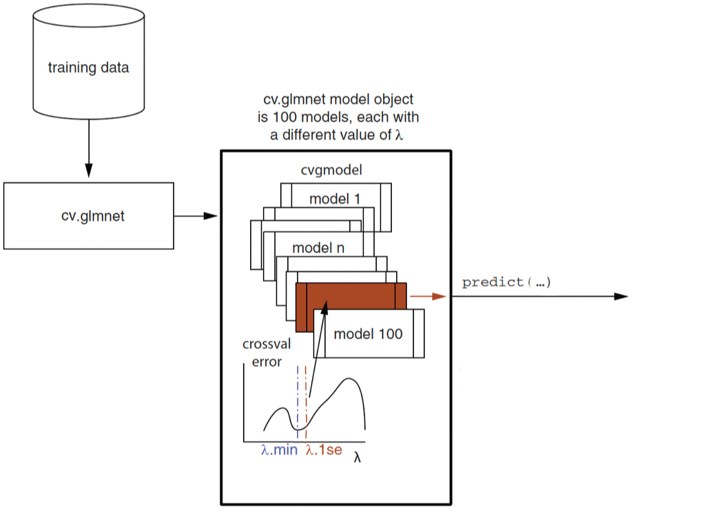
In a 7-fold cross-validated lasso logistic regression, how many logistic regression models does cv.glmnet() fit during the cross-validation process described above?
Show answer
In a 7-fold cross-validated lasso logistic regression, the model is fit once for each fold and each candidate value of \(\lambda\).
Since 100 lambda values are considered and there are 7 folds, the number of model fits during cross-validation is:
\(7 \times 100 = 700\)
So the answer is 700 logistic regression models.
Tip
Note: This is the main cross-validation count. In practice, cv.glmnet() may fit more than 700 models internally because it also fits the model on the full training data to construct the lambda sequence and summarize the final cross-validation results. So 700 is the standard counting answer, but the total internal number of fits can be a bit larger.
Q4h. Cross-Validated Regularization and Out-of-Sample Prediction
What is cross-validated regularization in regression modeling? Briefly explain why it can improve out-of-sample prediction.
Show answer
Cross-validated regularization means using cross-validation to choose the amount of regularization, such as the penalty parameter \(\lambda\), in a regression model.
Regularization shrinks coefficients and can reduce overfitting, while cross-validation helps choose the penalty that gives the best out-of-sample performance. This can improve out-of-sample prediction because it helps strike a good balance between underfitting and overfitting.
A model with no regularization may fit noise in the training data, while too much regularization may miss important patterns. Cross-validated regularization selects a level of complexity that tends to generalize better to new data.