install.packages("patchwork")
# remotes::install_github("thomasp85/patchwork")Reference 4
Combining Plots with patchwork
1 Introduction to patchwork
When building a data story, we often need to place multiple plots side by side, stack them vertically, or arrange them in a custom grid. Base R’s par(mfrow = ...) can do this for base graphics, but it does not work with ggplot2.
patchwork is the modern solution. It extends ggplot2 with a simple, expressive syntax for combining plots — using everyday operators like +, |, and /.
“The goal of patchwork is to make it ridiculously simple to combine separate ggplots into the same graphic.” — Thomas Lin Pedersen (package author)
1.1 Installation and loading
library(ggplot2)
library(patchwork)
2 Building Blocks — Four mtcars Plots
We create four plots from mtcars that we will combine in different ways throughout this lecture. Think of these as the building blocks.
p1 <- ggplot(mtcars) +
  geom_point(aes(mpg, disp), color = "steelblue") +
  labs(title = "Plot 1", x = "Miles per gallon", y = "Displacement")

p2 <- ggplot(mtcars) +
  geom_boxplot(aes(factor(gear), disp, fill = factor(gear)),
               show.legend = FALSE) +
  labs(title = "Plot 2", x = "Gears", y = "Displacement")

p3 <- ggplot(mtcars) +
  geom_point(aes(hp, wt, color = mpg)) +
  scale_color_viridis_c() +
  labs(title = "Plot 3", x = "Horsepower", y = "Weight")

p4 <- ggplot(mtcars) +
  geom_bar(aes(factor(gear), fill = factor(gear)),
           show.legend = FALSE) +
  facet_wrap(~cyl) +
  labs(title = "Plot 4", x = "Gears", y = "Count")
Display them individually to understand what each one shows before combining.
p1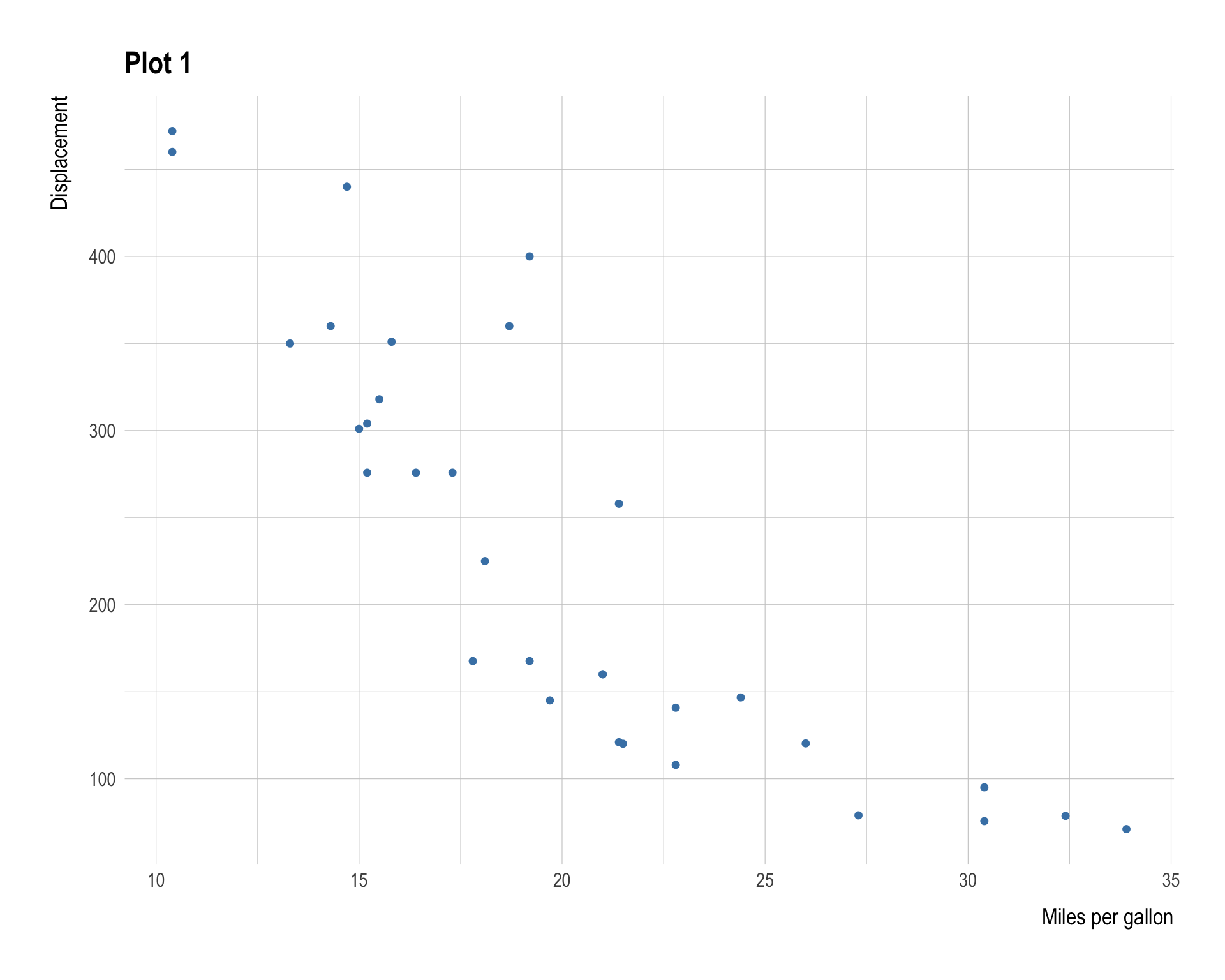
p2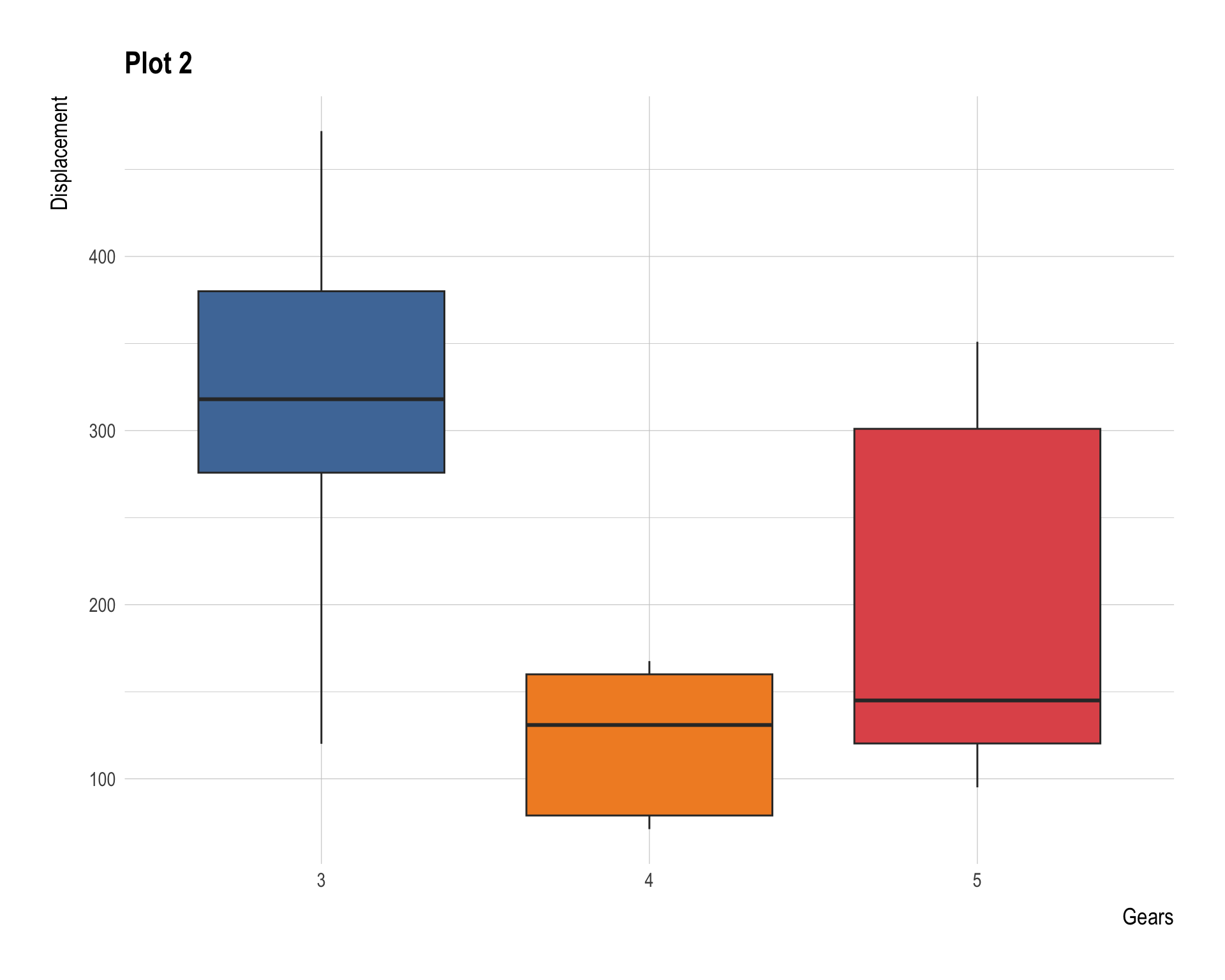
p3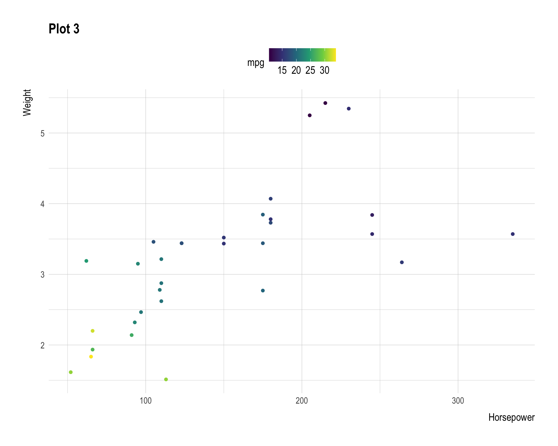
p4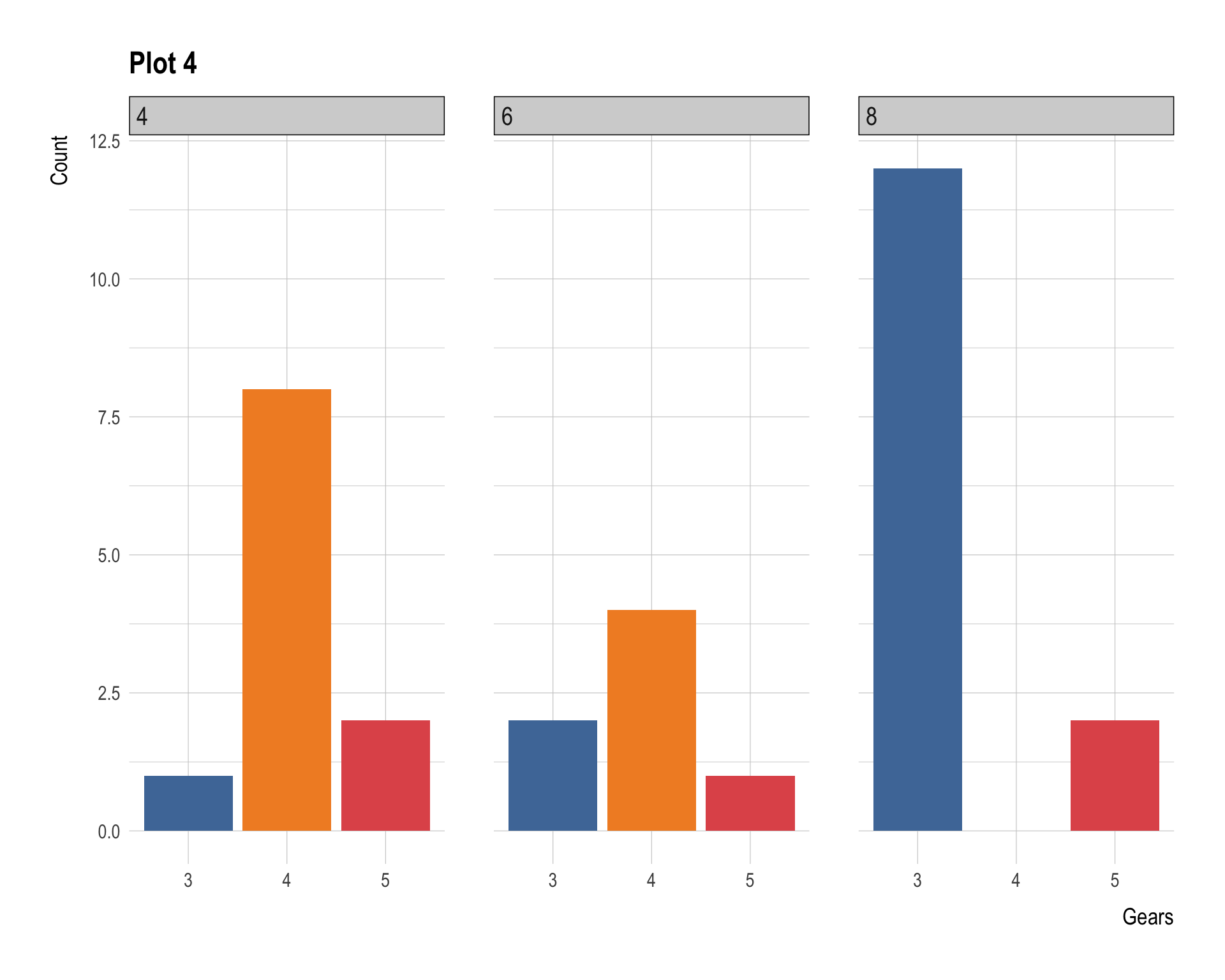
3 Basic Use — the + Operator
The simplest way to combine two plots is +. Patchwork places them side by side in a single row.
p1 + p2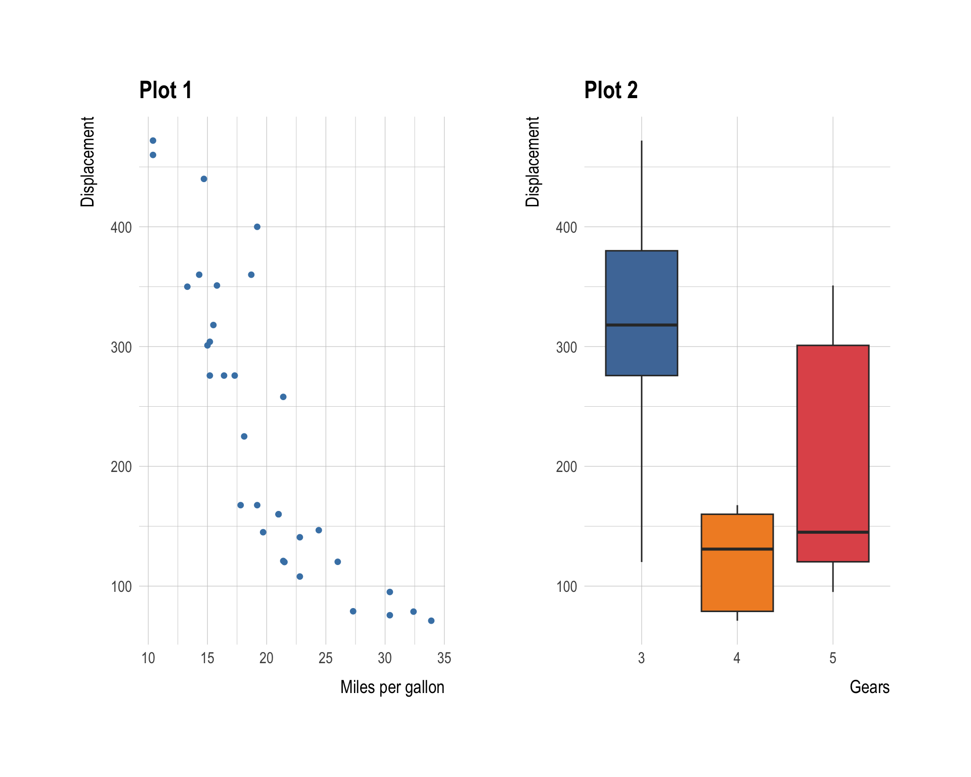
Note
The + operator is the same one used in ggplot2 to add layers, but when applied between two complete ggplot objects, patchwork intercepts it and creates a combined layout.
3.1 Additions flow to the last plot
When you add a ggplot2 element (such as labs()) after a patchwork, it is applied to the last plot in the composition:
p1 + p2 + labs(subtitle = "This subtitle appears in the last plot (p2)")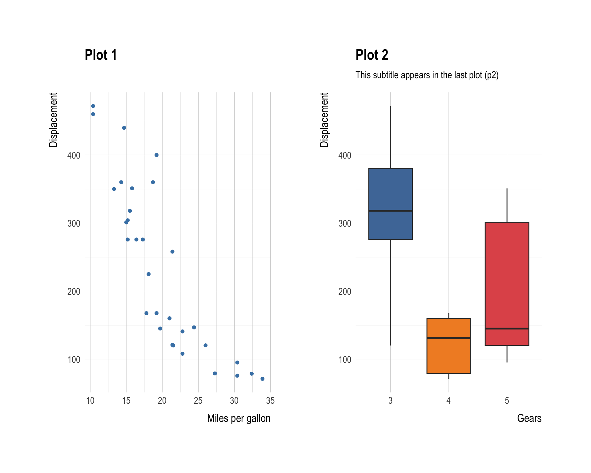
This is consistent with ggplot2’s own + semantics — keep it in mind to avoid accidental modifications.
4 Filling a Grid
Adding more than two plots fills a grid automatically. Patchwork tries to keep the grid as square as possible, filling in row-first order.
p1 + p2 + p3 + p4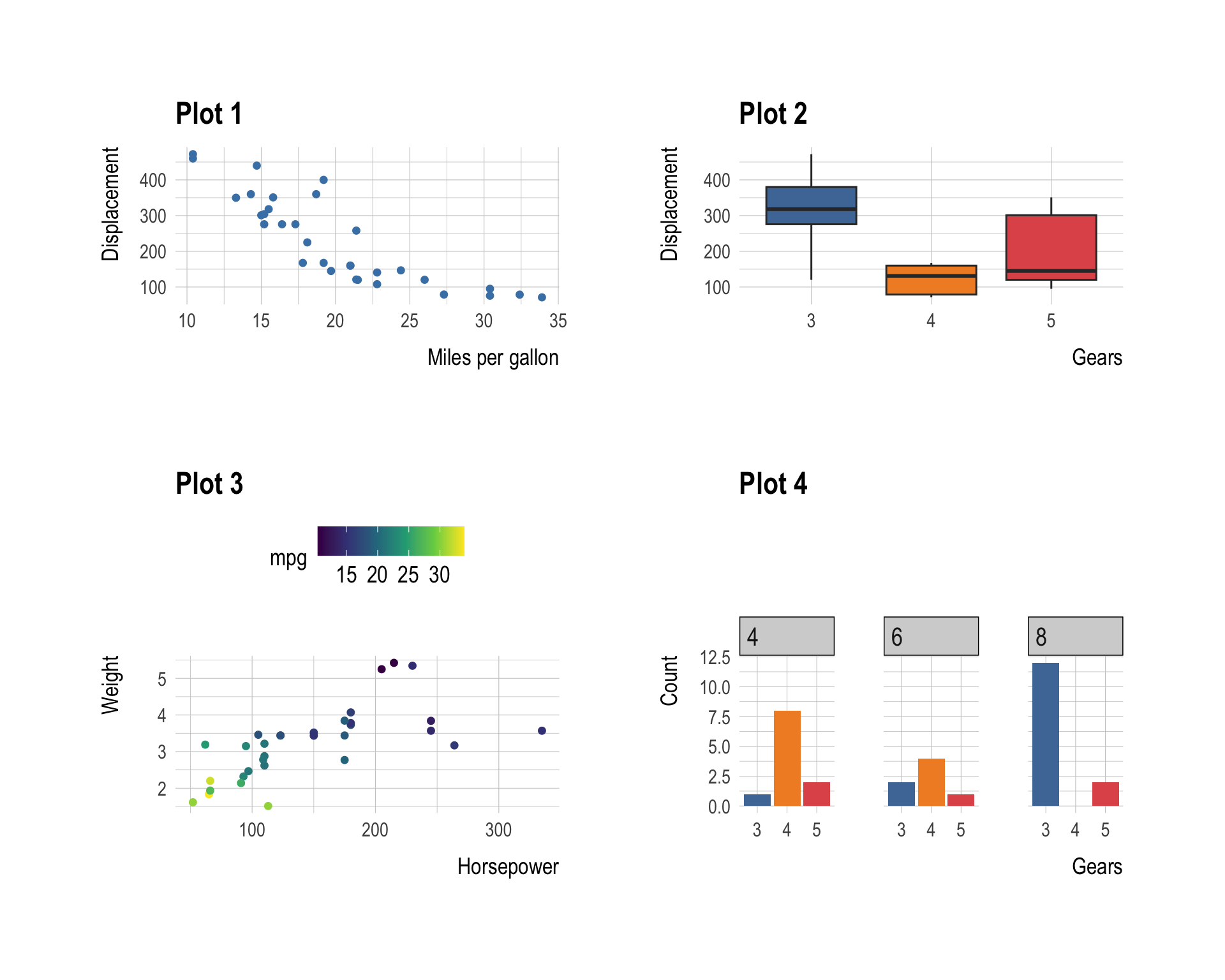
4.1 Controlling rows and columns with plot_layout()
Use plot_layout() to override the default grid dimensions.
p1 + p2 + p3 + p4 +
  plot_layout(nrow = 3, byrow = FALSE)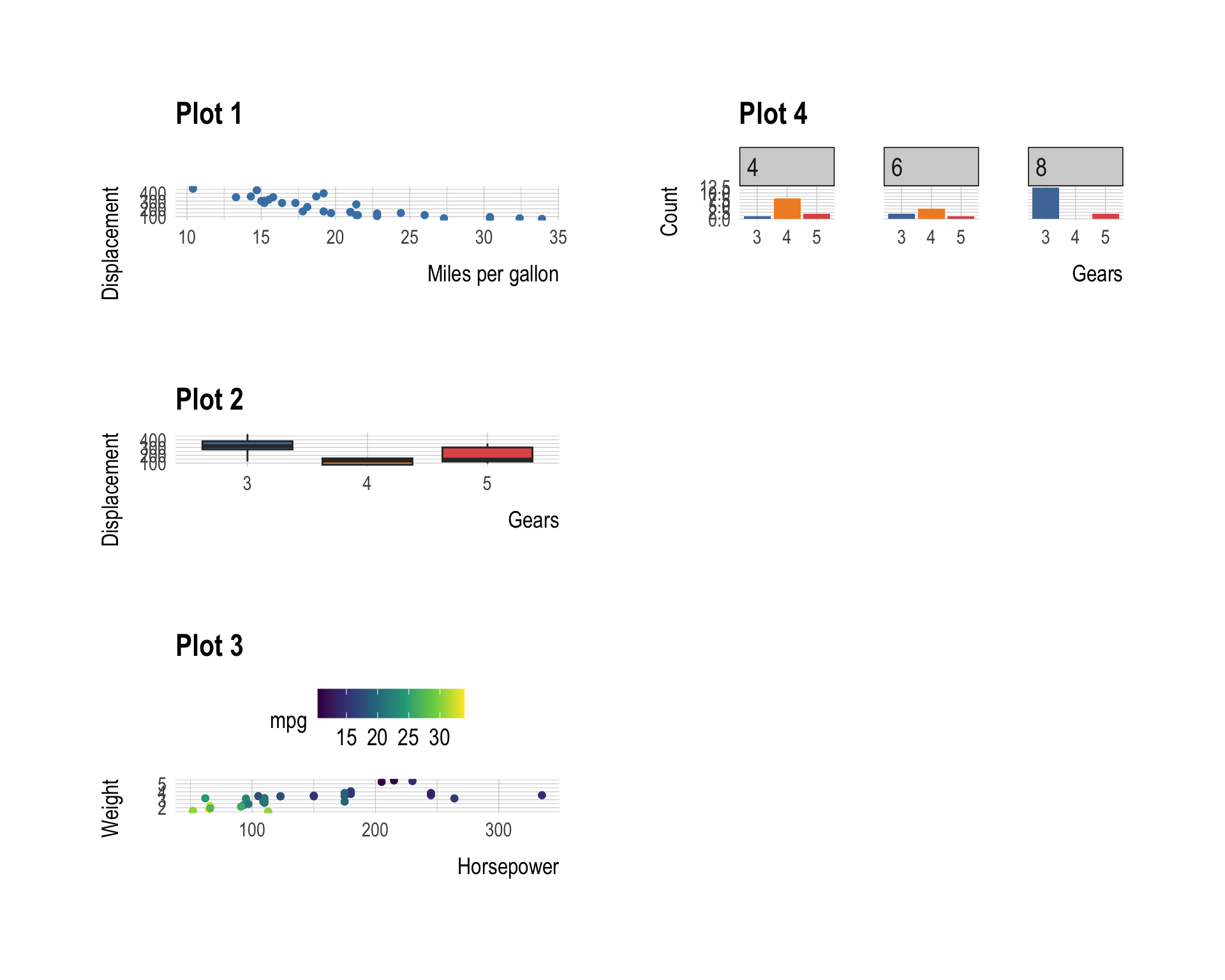
| Argument | Effect |
|---|---|
nrow |
Number of rows |
ncol |
Number of columns |
byrow |
Fill by row (TRUE) or column (FALSE) |
widths |
Relative widths of columns |
heights |
Relative heights of rows |
4.1.1 Relative sizing
Control how much space each column or row gets:
p1 + p2 + p3 +
  plot_layout(ncol = 3, widths = c(2, 1, 1))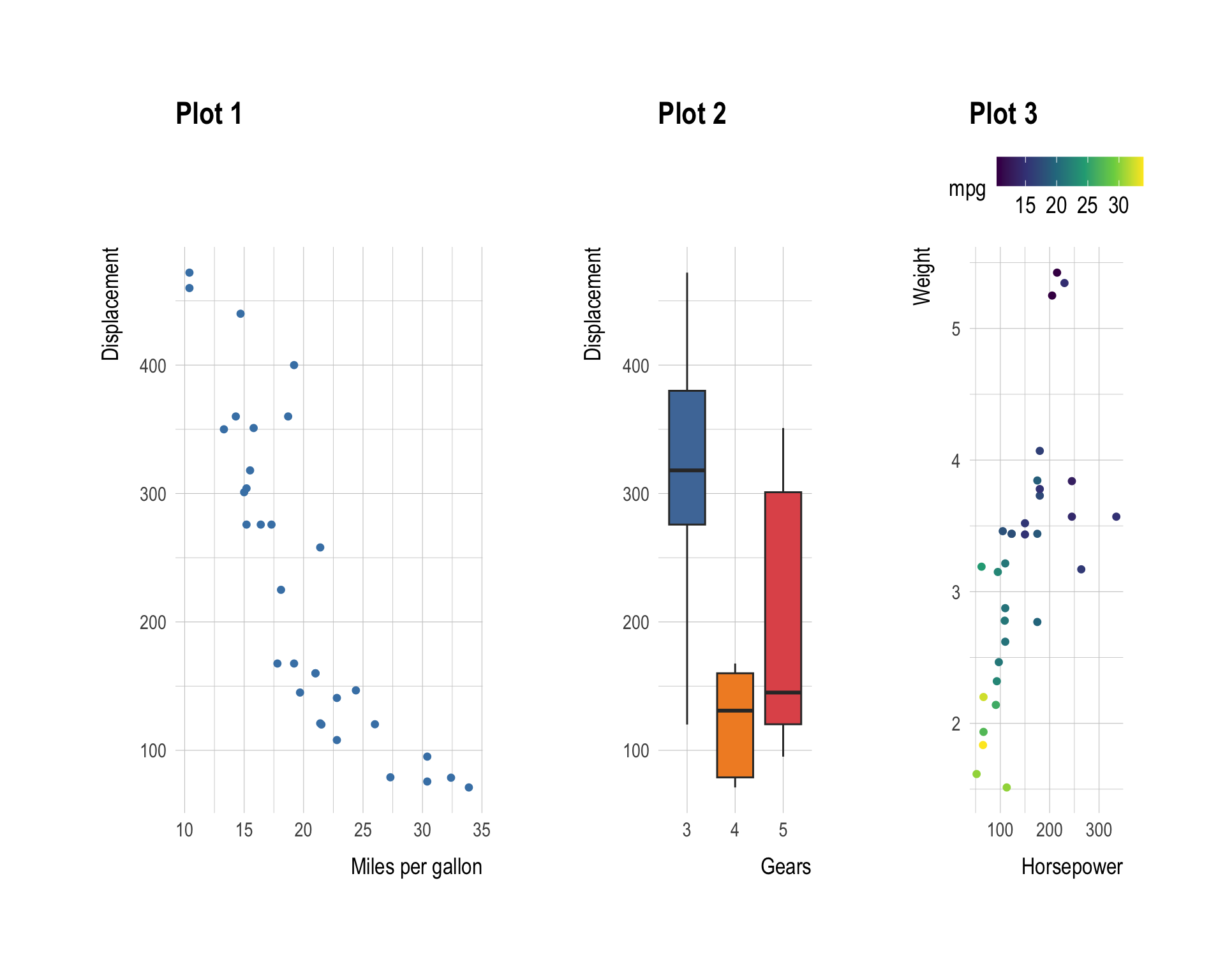
Here p1 gets twice as much horizontal space as p2 and p3.
5 Stacking and Placing Side by Side
patchwork provides two dedicated operators for the two most common layouts:
| Operator | Layout |
|---|---|
\| |
Place plots beside each other (same row) |
/ |
Stack plots on top of each other (same column) |
5.1 Side by side with |
p1 | p2
5.2 Stacked with /
p1 / p2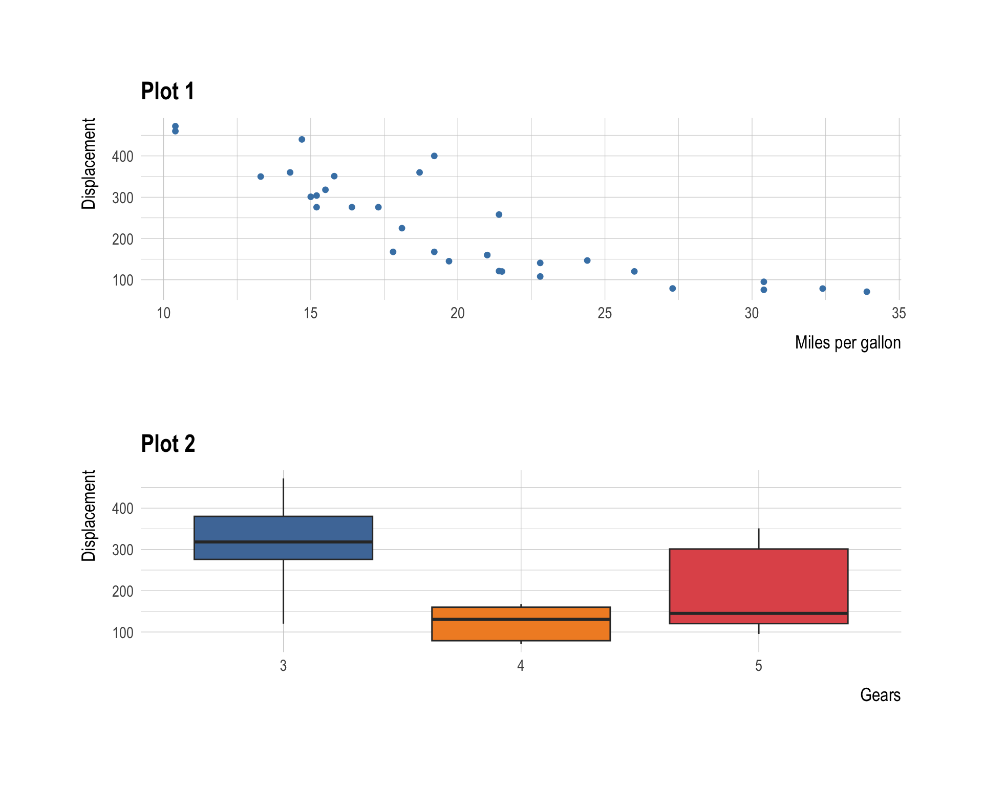
6 Nesting Layouts
Because | and / return patchwork objects themselves, they can be nested using parentheses to create complex multi-panel figures.
6.1 One column beside a stacked pair
p1 | (p2 / p3)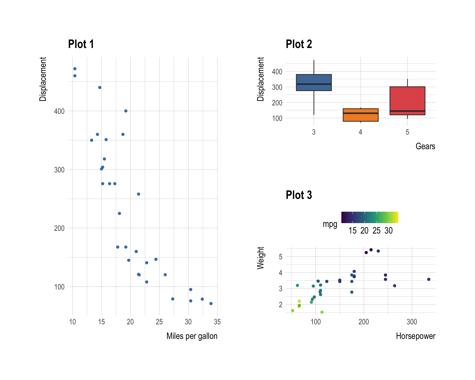
6.2 A stacked pair beside another plot
(p1 / p2) | p3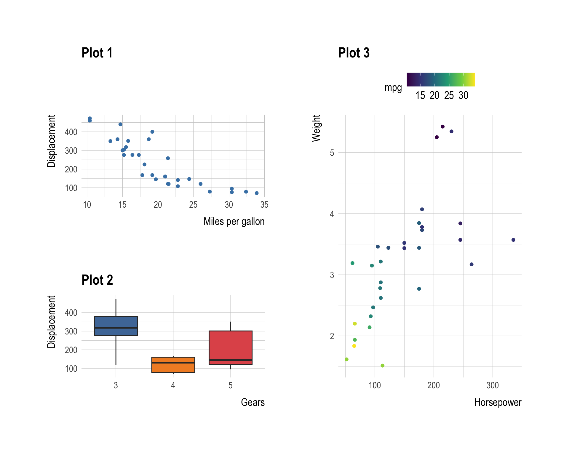
6.3 Three-level nesting
p1 | (p2 / (p3 | p4))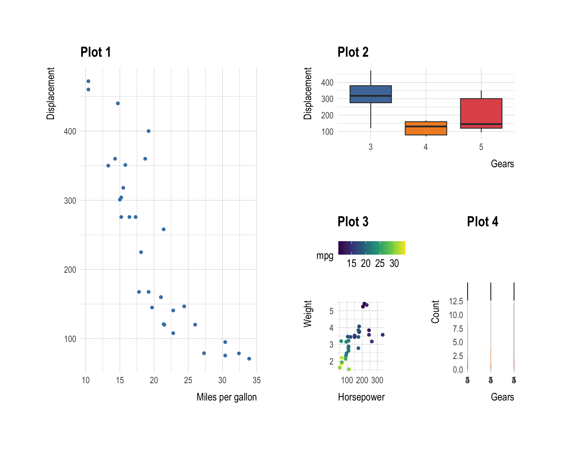
Tip
Reading nested patchwork expressions — evaluate the innermost parentheses first, just like arithmetic. p3 | p4 is a row, p2 / (p3 | p4) stacks p2 above that row, and finally p1 | ... places p1 to the left of the whole thing.
7 Annotating a Composition
A combined figure often needs a shared title, subtitle, caption, or tagged subplot labels. Use plot_annotation() for this.
7.1 Shared title and caption
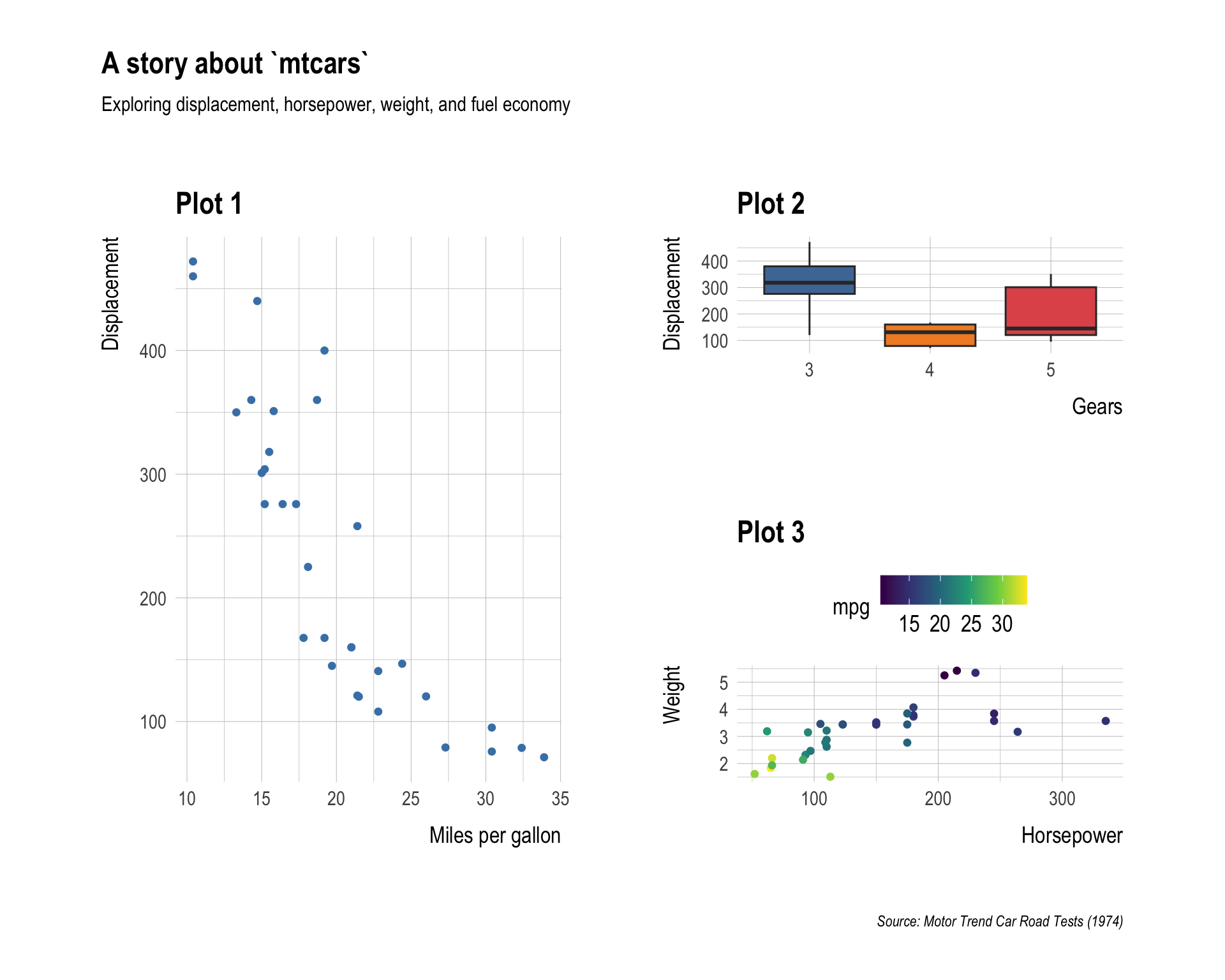
(p1 | (p2 / p3)) +
  plot_annotation(
    title   = "A story about `mtcars`",
    subtitle = "Exploring displacement, horsepower, weight, and fuel economy",
    caption  = "Source: Motor Trend Car Road Tests (1974)"
  )
7.2 Auto-tagging subplots
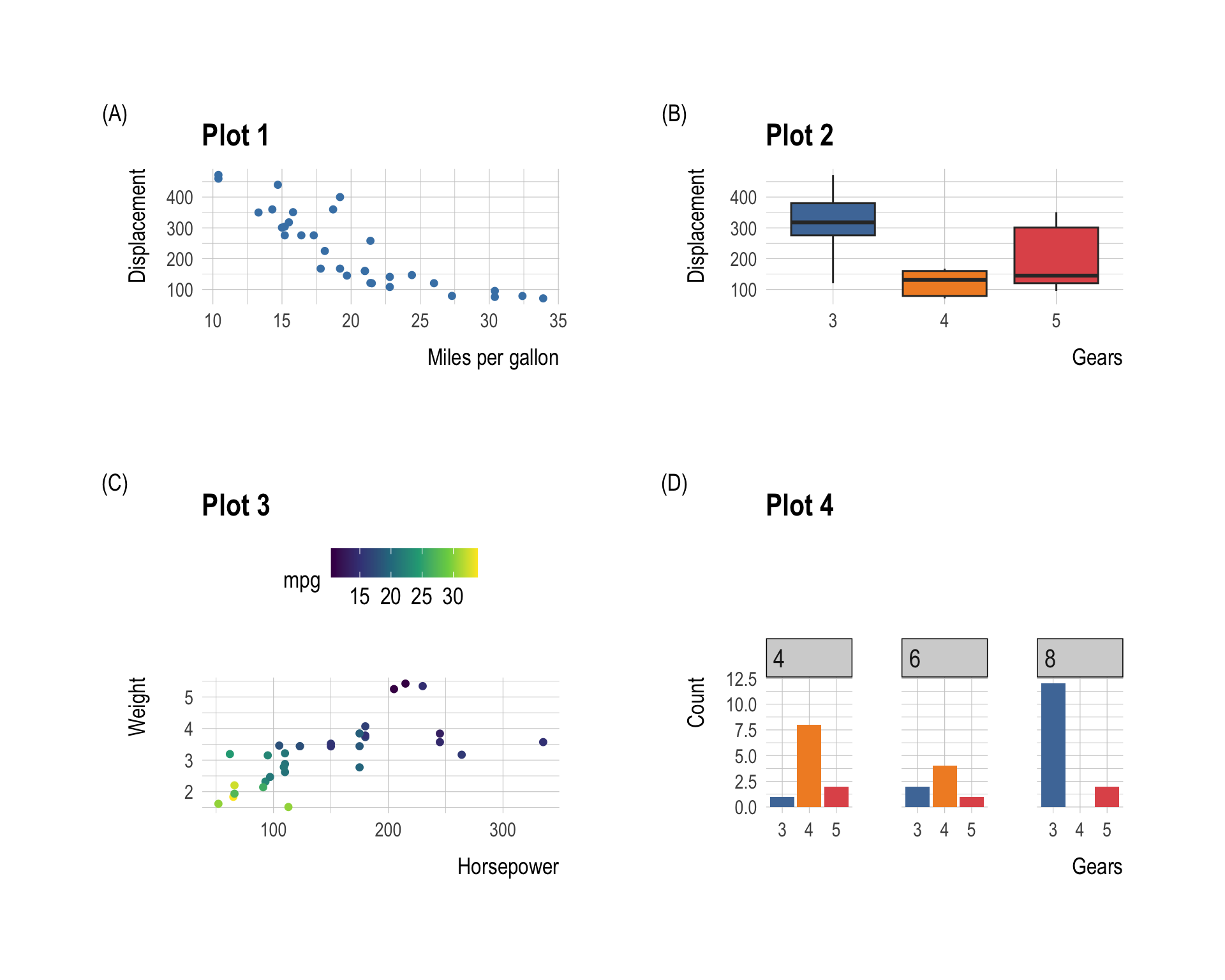
Patchwork can automatically label each panel so you can refer to them in text as (A), (B), etc.
p1 + p2 + p3 +
  plot_annotation(tag_levels = "A")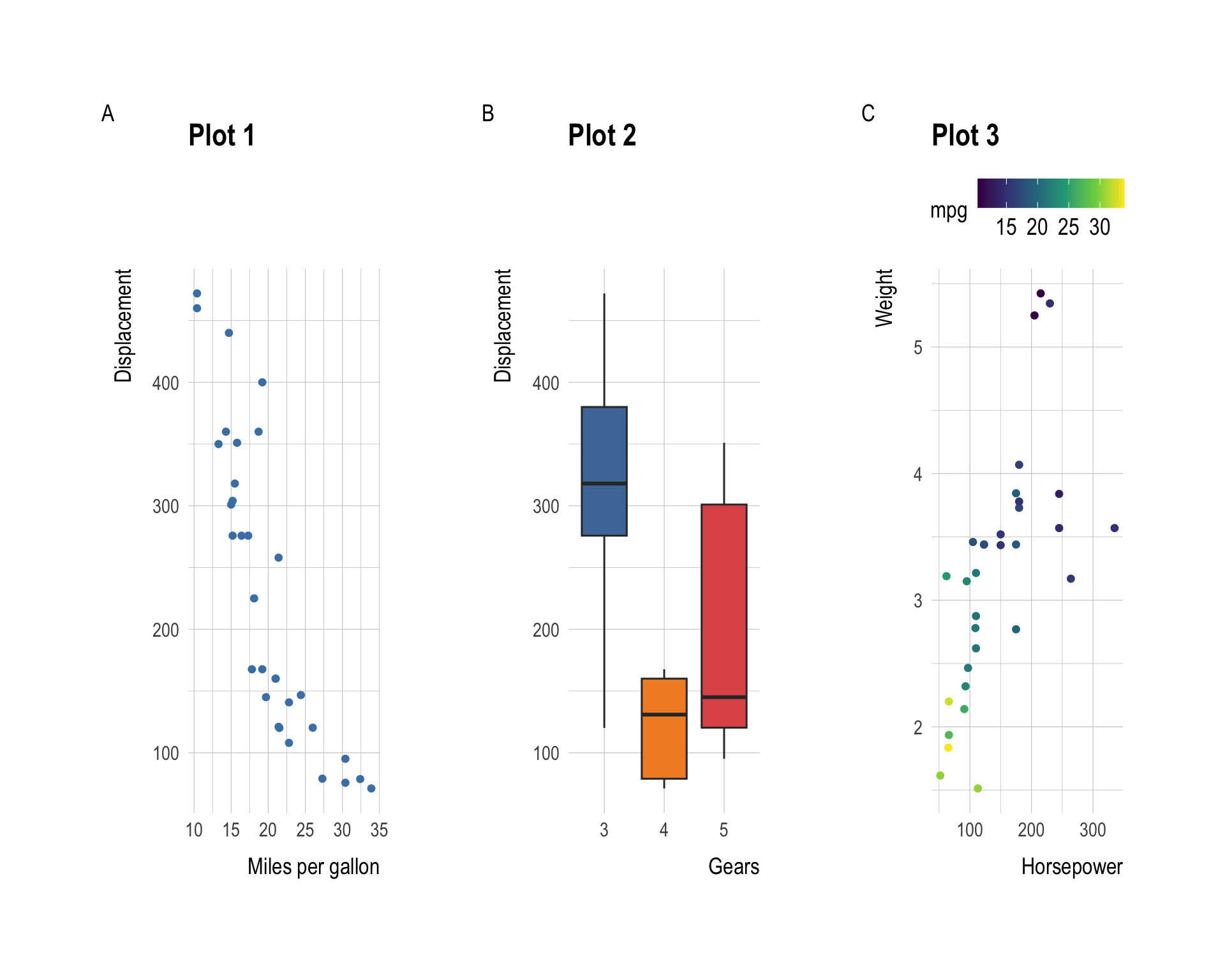
Available tag styles:
tag_levels |
Labels |
|---|---|
"A" |
A, B, C, … |
"a" |
a, b, c, … |
"1" |
1, 2, 3, … |
"I" |
I, II, III, … |
"i" |
i, ii, iii, … |
p1 + p2 + p3 + p4 +
  plot_annotation(tag_levels = "I")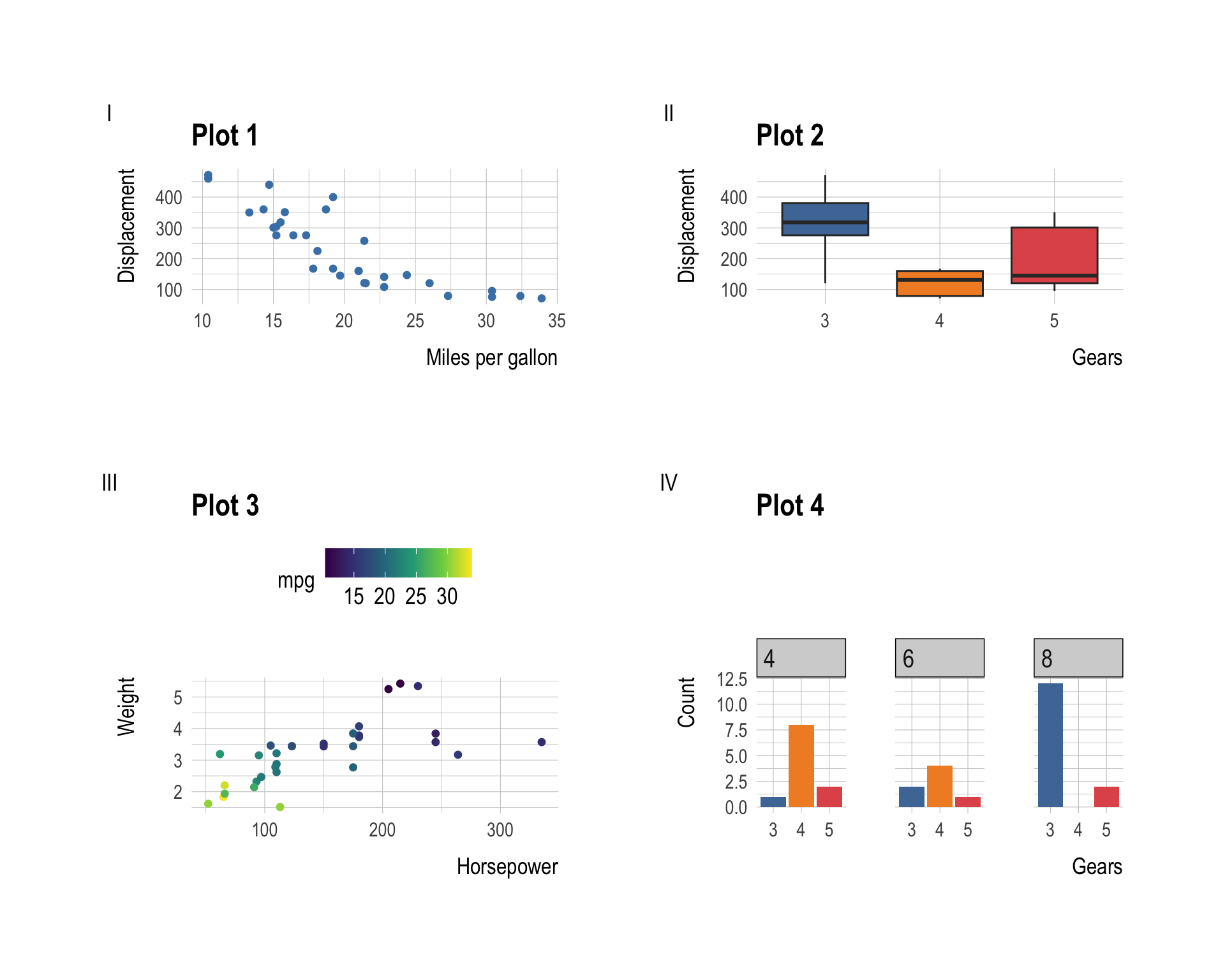
7.3 Styling tags with tag_prefix and tag_suffix
p1 + p2 + p3 + p4 +
  plot_annotation(
    tag_levels = "A",
    tag_prefix = "(",
    tag_suffix = ")"
  )
8 Modifying Individual Panels in a Composition
After combining plots, you can still apply ggplot2 modifications to a specific panel using [[i]] indexing.
combined <- p1 + p2 + p3

# Change the theme of the second panel only
combined[[2]] <- combined[[2]] + theme_minimal()

combined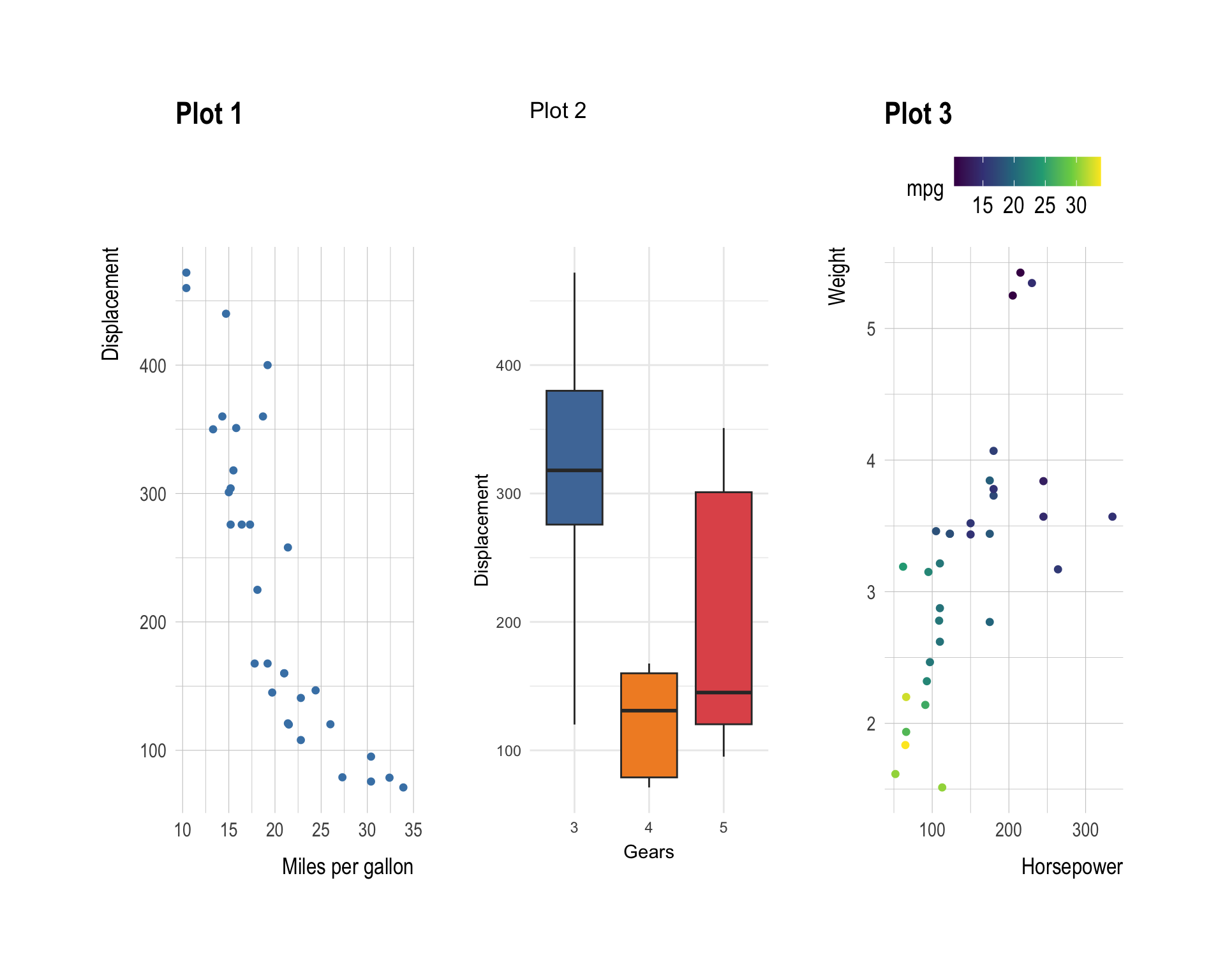
9 Collecting Legends
When multiple panels share the same aesthetic (e.g., the same color scale), their legends are redundant. Use plot_layout(guides = "collect") to merge them into one.
# Two plots that both use fill = factor(cyl)
q1 <- ggplot(mtcars) +
  geom_point(aes(mpg, disp, color = factor(cyl))) +
  labs(title = "mpg vs. disp", color = "Cylinders")

q2 <- ggplot(mtcars) +
  geom_point(aes(hp, wt, color = factor(cyl))) +
  labs(title = "hp vs. wt", color = "Cylinders")

q1 + q2 + plot_layout(guides = "collect")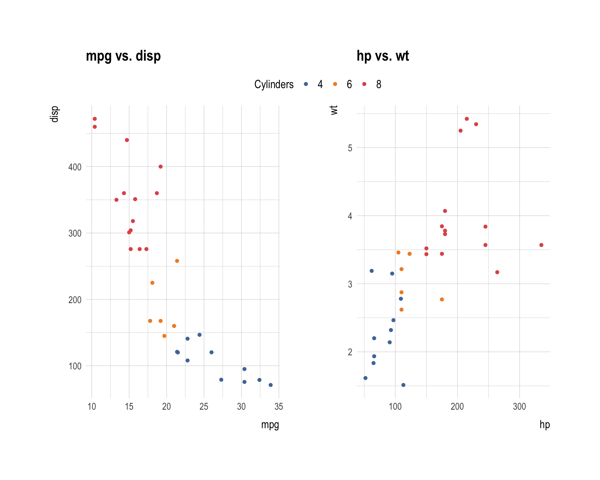
Without guides = "collect", each panel carries its own legend — cluttering the figure. With it, the legend is deduplicated and placed at the right edge by default.
10 Adding Empty Space with plot_spacer()
Sometimes you want a blank cell in your grid (e.g., to shift a plot to the right or leave room for a manual annotation). Use plot_spacer():
p1 + plot_spacer() + p2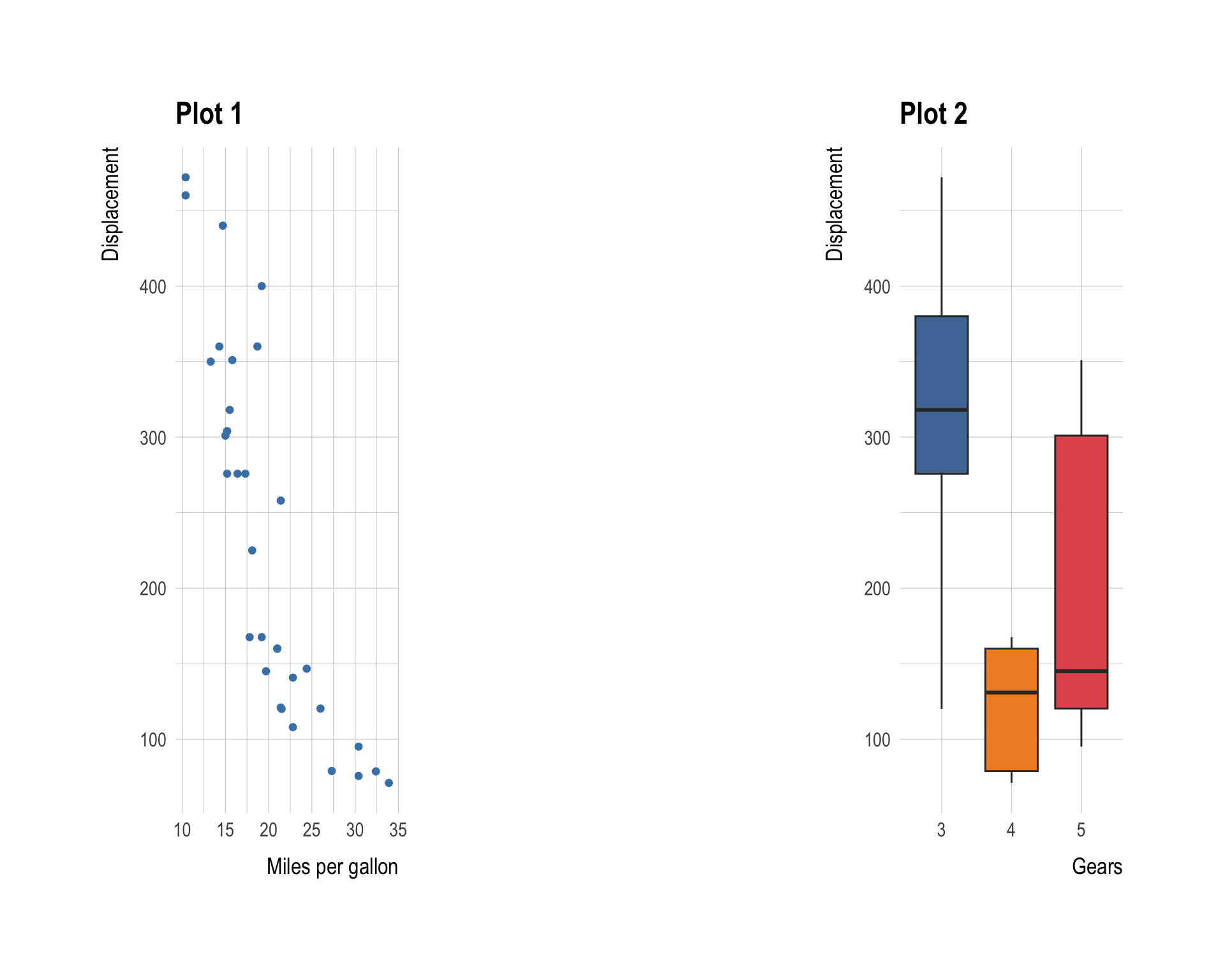
# Place p3 in the bottom-right of a 2x2 grid
plot_spacer() + plot_spacer() + plot_spacer() + p3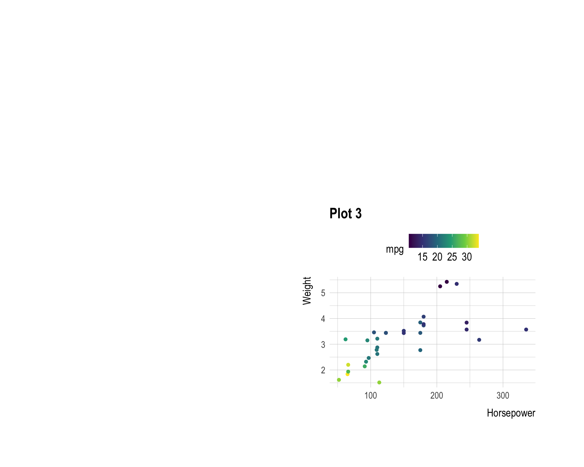
11 Insets with inset_element()
inset_element() places one plot on top of another as an inset — like a zoomed-in detail or a small map overlay.
p3 + inset_element(p1, left = 0.6, bottom = 0.6, right = 1, top = 1)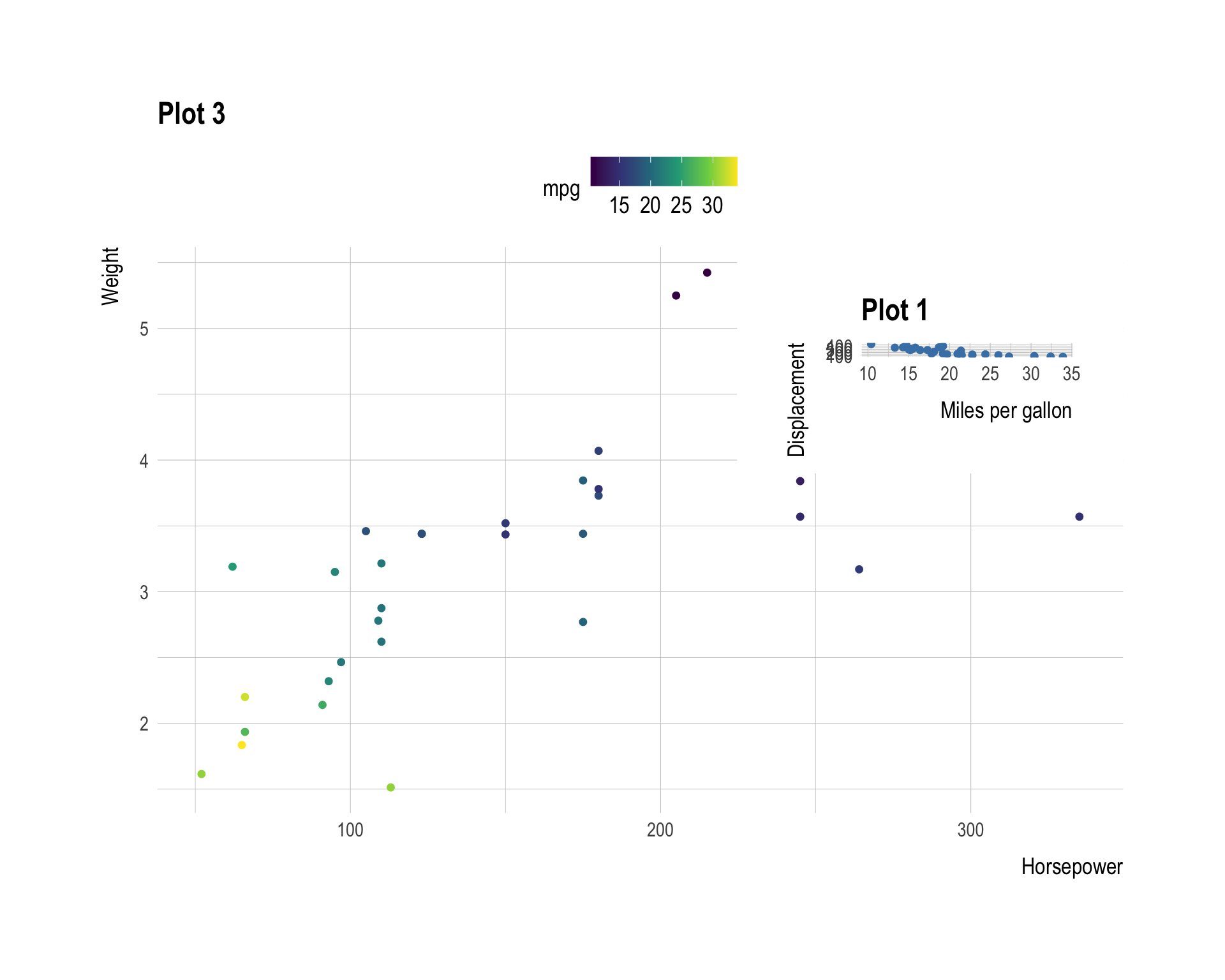
The left, right, bottom, and top arguments are proportions of the base plot’s area (0 to 1). Here the inset occupies the upper-right 40% × 40% of p3.
12 Putting It All Together — A Publication-Ready Figure
Combining all the tools we have learned: nested layouts, collected legends, auto-tags, and a shared annotation.
final_figure <-
  ((q1 | q2) / (p2 | p4)) +
  plot_layout(guides = "collect") +
  plot_annotation(
    title    = "Motor Trend Car Road Tests — `mtcars` Overview",
    subtitle = "Top row: continuous relationships by cylinder count | Bottom row: discrete summaries",
    caption  = "Data: Motor Trend (1974)",
    tag_levels = "A",
    tag_prefix = "(",
    tag_suffix = ")"
  ) &
  theme_minimal(base_size = 11)

final_figure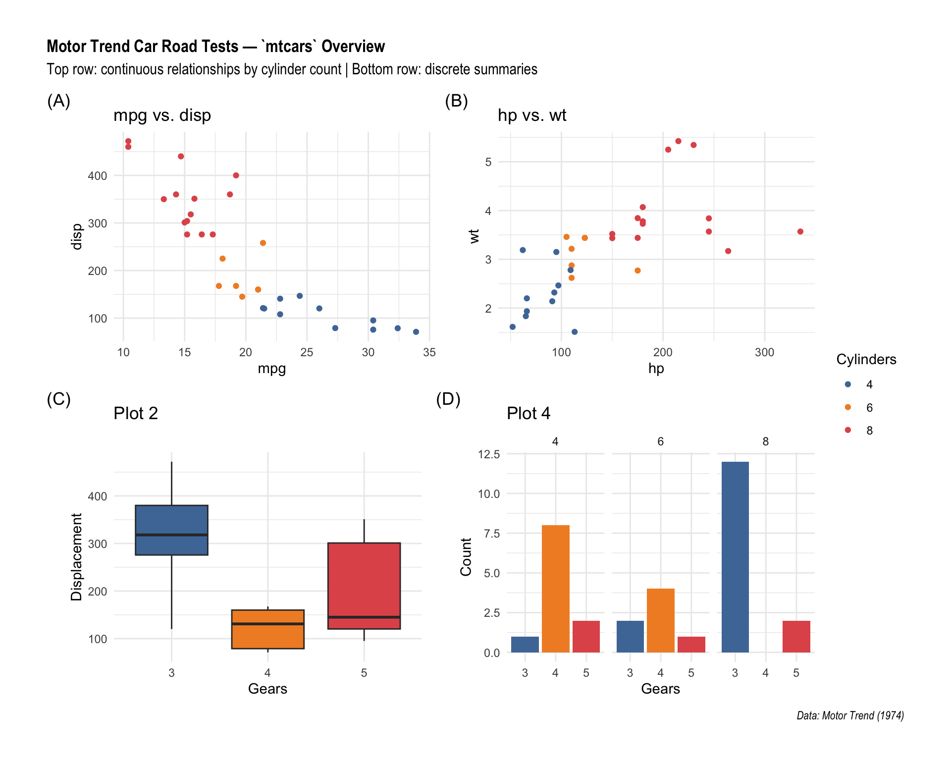
The
& operator
& theme_minimal() applies a theme to all panels at once, unlike + which only targets the last panel. Use & whenever you want a global style change across every plot in a patchwork.
13 Quick Reference
| Task | Code |
|---|---|
| Place side by side | p1 \| p2 |
| Stack vertically | p1 / p2 |
| Fill a 2×2 grid | p1 + p2 + p3 + p4 |
| Control rows/cols | + plot_layout(nrow = 2) |
| Relative widths | + plot_layout(widths = c(2, 1)) |
| Shared title/caption | + plot_annotation(title = "...") |
| Auto-tag panels | + plot_annotation(tag_levels = "A") |
| Collect legends | + plot_layout(guides = "collect") |
| Blank cell | plot_spacer() |
| Inset plot | + inset_element(p, left, bottom, right, top) |
| Style all panels | & theme_minimal() |
| Modify one panel | combined[[2]] <- combined[[2]] + ... |
14 Further Reading
- patchwork documentation
- Plot Assembly guide —
wrap_plots(),wrap_elements(), nesting details - Controlling Layouts —
area(), complex grid specifications - Annotation and Style — per-level tagging, theme control
- Multi-page Alignment — aligning panels across
gridandcowplotpages