Final Exam

DANL 101

Section 3. Data Analysis with R

Question 25

Consider the following vector x:

x <- c(2, 4, 6, 8, 10)

Write the R code to create a new vector called z, where its \(i\)-th entry (\(i = 1,2,3,4, \text{or } 5\)) is the standardized value of \(i\)-th element of x vector.

\[ z_{i} = \frac{x_{i} - \bar{x}}{\sigma_{x}} \]

• \(\bar{x}\): the mean of values in x
• \(\sigma_{x}\): the standard deviation of values in x

Answer: ______________________________________

Show answer

z <- (x - mean(x)) / sd(x)

Question 26

Given the data.frame df with variables height and name, which of the following expressions returns a vector containing the values in the height variable?

1. df:height
2. df$height
3. df::height
4. Both b and c

Show answer

b. df$height

Question 27

Consider the following data.frame, students:

Name	Age	Major	GPA
Alice	22	Business Administration	3.8
Bob	23	Accounting	3.2
Charlie	21	Data Analytics	3.9
Diana	24	Economics	3.5

Which of the following R codes will correctly create a new data.frame with only the Name and GPA variables?

1. students |> select(Name, GPA)
2. students |> select(-Age, -Major)
3. Both a and b

Show answer

c. Both a and b

Question 28

Consider the following data.frame df0:

x	y
Na	7
2	NA
3	9

What is the result of median(df0$y)?

1. 7
2. NA
3. 8
4. 9

Show answer

b. NA

Question 29

Consider the two related data.frames, df_1 and df_2:

• df_1

id	name	age
1	Bob	19
2	Julia	21
4	Zachary	20

• df_2

id	major
1	Economics
2	Business Administration
3	Data Analytics

Which of the following R code correctly join the two related data.frames, df_1 and df_2, to produce the resulting data.frame shown below?

id	name	age	major
1	Bob	19	Economics
2	Julia	21	Business Administration
4	Zachary	20	NA

1. df_1 |> left_join(df_2)
2. df_2 |> left_join(df_1)
3. Both a and b
4. None of the above

Show answer

a. df_1 |> left_join(df_2)

Questions 30-36

For Questions 30-36, consider the following R packages and the data.frame, nyc_dogs, containing individual dog license data from New York City (NYC):

library(tidyverse)
library(skimr)
library(ggthemes)

nyc_dogs <- read_csv("https://bcdanl.github.io/data/nyc_dogs_cleaned.csv")

The first 10 observations in the nyc_dogs data frame are displayed below:

name	gender	birth_year	breed	borough
paige	F	2014	pit bull	Manhattan
yogi	M	2010	boxer	Bronx
ali	M	2014	basenji	Manhattan
queen	F	2013	akita	Manhattan
lola	F	2009	maltese	Manhattan
ian	M	2006	NA	Manhattan
buddy	M	2008	NA	Manhattan
chewbacca	F	2012	labrador	Manhattan
heidi-bo	F	2007	dachshund smooth coat	Brooklyn
massimo	M	2009	bull dog, french	Brooklyn

• The nyc_dogs data frame is with 197473 observations and 5 variables.

Description of Variables in nyc_dogs:

• name: Dog name

• gender: Dog gender (F for female; M for male; NA for missing value)

• birth_year: Birth year (integer values)

• breed: Dog breed

• borough: Borough in NYC

The followings are the summary of the nyc_dogs data.frame, including descriptive statistics for each variable.

Data summary

Name	nyc_dogs
Number of rows	197473
Number of columns	5
_______________________
Column type frequency:
character	4
numeric	1
________________________
Group variables	None

Variable type: character

skim_variable	n_missing	min	max	empty	n_unique
name	2637	1	30	0	26770
gender	6	1	1	0	2
breed	18832	3	35	0	295
borough	0	5	13	0	5

Variable type: numeric

skim_variable	n_missing	mean	sd	p0	p25	p50	p75	p100
birth_year	0	2012.94	4.91	1975	2010	2014	2017	2021

Question 30

What is the interquartile range of birth_year? Find this value by using the summary of the nyc_dogs data frame.

---

Show answer

IQR = 7 = 2017 - 2010

Question 31

What R code can we use to count the number of licensed dogs by borough within each birth_year in NYC?

1. nyc_dogs |> count(birth_year)
2. nyc_dogs |> count(borough)
3. nyc_dogs |> count(borough, birth_year)
4. nyc_dogs |> count(birth_year, borough)
5. Both c and d

Show answer

e

Question 32

• We are interested in finding the 7 most popular dog breeds in NYC.
• To achieve this, we create a new data.frame, a new data.frame, top7_breeds, which includes only 7 most popular dog breeds, excluding any NA values.

breed	n
yorkshire terrier	12804
shih tzu	12790
chihuahua	11099
labrador	11017
pit bull	10023
maltese	7750
german shepherd	5063

• The top7_breeds data.frame is displayed above.

top7_breeds <- nyc_dogs |> 
  filter(___(1)___) |> 
  ___(2)___ |> 
  ___(3)___(-n) |> 
  head(7)  # returns the first 7 observations of the new data.frame

• Complete the code by filling in the blanks (1)-(3).

1. 1. is.na(breed); (2) count(n); (3) select
2. 1. is.na(breed); (2) count(n); (3) arrange
3. 1. is.na(breed); (2) count(breed); (3) select
4. 1. is.na(breed); (2) count(breed); (3) arrange
5. 1. !is.na(breed); (2) count(n); (3) select
6. 1. !is.na(breed); (2) count(n); (3) arrange
7. 1. !is.na(breed); (2) count(breed); (3) select
8. 1. !is.na(breed); (2) count(breed); (3) arrange

Show answer

h

Question 33

How would you describe the distribution of breed using the top7_breeds data.frame?

• Note that the breed categories are sorted by the n variable in the plot.

Complete the code by filling in the blanks (1)-(3).

ggplot(data = top7_breeds,
       mapping = aes(___(1)___,
                     ___(2)___ = n)) +
  ___(3)___() +
  labs(y = "Top 7 Dog Breeds")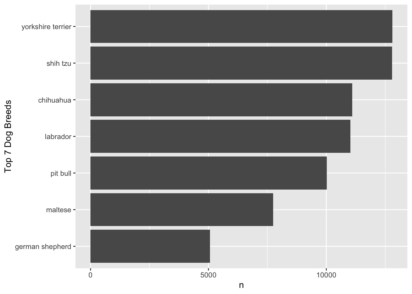

Blank (1)

1. x = breed
2. y = breed
3. x = fct_reorder(n, breed)
4. y = fct_reorder(n, breed)
5. x = fct_reorder(breed, n)
6. y = fct_reorder(breed, n)
7. Both c and d
8. Both e and f

Show answer

f

Blank (2)

1. x
2. y
3. fill
4. color

Show answer

a

Blank (3)

1. geom_bar
2. geom_col
3. Both a and b

Show answer

b

Question 34

• We are also interested in identifying the top five most popular dog names for each gender.
• To do this, we first create a new data frame, nyc_dogs_filtered, which includes only the observations where (1) the value of name variable is not missing and (2) the value of gender variable is not missing.

nyc_dogs_filtered <- nyc_dogs |> 
  filter(___BLANK___)

• Which condition correctly fills in the BLANK to complete the code above?

1. is.na(name) , is.na(gender)
2. is.na(name) & is.na(gender)
3. is.na(name) | is.na(gender)
4. !is.na(name) , !is.na(gender)
5. !is.na(name) & !is.na(gender)
6. !is.na(name) | !is.na(gender)
7. Both a and b
8. Both a and c
9. Both d and e
10. Both d and f

Show answer

i

Question 35

• Using nyc_dogs_filtered from Question 34, we are creating the top5names_F data.frame:

name	n
bella	1291
lola	1005
luna	995
lucy	914
daisy	851

• The top5names_F data.frame provides the five most popular female dog names, displayed above.

Complete the code by filling in the blanks (1)-(2).

top5names_F <- nyc_dogs_filtered |> 
  filter(___(1)___) |> 
  count(___(2)___) |> 
  arrange(___(3)___) |> 
  head(5) 

Blank (1)

1. gender == "F"
2. gender != "F"
3. gender == "M"
4. gender != "M"
5. Both a and b
6. Both a and c
7. Both a and d
8. Both b and c
9. Both b and d
10. Both c and d

Show answer

g

Blank (2)

1. name
2. gender
3. n
4. name, n
5. gender, n
6. name, gender
7. gender, name

Show answer

a

Blank (3)

1. n
2. -n
3. desc(n)
4. Both b and c

Show answer

d

Question 36

• Likewise, using nyc_dogs_filtered from Question 34, we are creating the top5names_M data.frame:

name	n
max	1341
charlie	1042
rocky	1020
buddy	840
teddy	745

• The top5names_M data.frame provides the five most popular male dog names, displayed above.

Complete the code by filling in the blanks (1)-(2).

top5names_M <- nyc_dogs_filtered |> 
  filter(___(1)___) |> 
  count(___(2)___) |> 
  arrange(___(3)___) |> 
  head(5) 

Blank (1)

1. gender == "F"
2. gender != "F"
3. gender == "M"
4. gender != "M"
5. Both a and b
6. Both a and c
7. Both a and d
8. Both b and c
9. Both b and d
10. Both c and d

Show answer

h

Blank (2)

1. name
2. gender
3. n
4. name, n
5. gender, n
6. name, gender
7. gender, name

Show answer

a

Blank (3)

1. n
2. -n
3. desc(n)
4. Both b and c

Show answer

d

Questions 37-40

The Nobel Prize in Economic Science in 2021 goes to David Card, Joshua Angrist and Guido Imbens, for their empirical contributions to labor economics, and for their methodological contributions to the analysis of causal relationships.

They have provided us with new insights about the labor market and shown what conclusions about cause and effect can be drawn from natural experiments. Their approach has spread to other fields and revolutionized empirical research.

For Questions 37-40, consider the following R packages and the data.frame, ak91_age, which comes from the 1980 US Census and covers men born 1930–1939, which is used by Joshua Angrist and Alan Krueger’s research article.

library(tidyverse)
library(skimr)
library(ggthemes)

ak91_age <- read_csv('https://bcdanl.github.io/data/ak91_ageW.csv')

The first 20 observations in the ak91_age data frame are displayed below:

QoB	YoB	YoBQ	W	Educ	Q4
1	1930	1930.00	361.0922	12.28041	FALSE
1	1931	1931.00	365.8181	12.54043	FALSE
1	1932	1932.00	364.9678	12.53393	FALSE
1	1933	1933.00	362.1093	12.67319	FALSE
1	1934	1934.00	363.2739	12.64726	FALSE
1	1935	1935.00	357.7532	12.65091	FALSE
1	1936	1936.00	359.5803	12.74304	FALSE
1	1937	1937.00	362.5073	12.83230	FALSE
1	1938	1938.00	362.9918	12.93868	FALSE
1	1939	1939.00	360.0860	13.00299	FALSE
2	1930	1930.25	364.3105	12.42842	FALSE
2	1931	1931.25	365.2228	12.53105	FALSE
2	1932	1932.25	365.2356	12.60960	FALSE
2	1933	1933.25	365.2171	12.63471	FALSE
2	1934	1934.25	362.2778	12.72797	FALSE
2	1935	1935.25	360.1939	12.79693	FALSE
2	1936	1936.25	360.2046	12.81108	FALSE
2	1937	1937.25	360.7164	12.84405	FALSE
2	1938	1938.25	366.8558	13.00766	FALSE
2	1939	1939.25	365.9290	13.01340	FALSE

• The ak91_age data frame is with 40 observations and 6 variables.

Description of Variables in ak91_age:

• QoB: Quarter of birth
• YoB: Year of birth (1930, 1931, …, 1939)
• YoBQ: Year and quarter of birth (1930 Q1, 1930 Q2, …, 1939 Q4)
• W: Wage per week
• Educ: Years of education
• Q4: TRUE if quarter of birth is 4; FALSE otherwise.

The followings are the summary of the ak91_age data.frame, including descriptive statistics for each variable.

Data summary

Name	ak91_age
Number of rows	40
Number of columns	6
_______________________
Column type frequency:
logical	1
numeric	5
________________________
Group variables	None

Variable type: logical

skim_variable	n_missing	mean	count
Q4	0	0.25	FAL: 30, TRU: 10

Variable type: numeric

skim_variable	n_missing	mean	sd	p0	p25	p50	p75	p100
QoB	0	2.50	1.13	1.00	1.75	2.50	3.25	4.00
YoB	0	1934.50	2.91	1930.00	1932.00	1934.50	1937.00	1939.00
YoBQ	0	1934.88	2.92	1930.00	1932.44	1934.88	1937.31	1939.75
W	0	365.02	3.37	357.75	362.24	365.53	367.89	370.32
Educ	0	12.76	0.19	12.28	12.64	12.75	12.93	13.12

Question 37

Here we describe the quarterly trend of years of education. Complete the code by filling in the blanks (1)-(3).

ggplot(data = ak91_age, 
       mapping = aes(___(1)___,
                     ___(2)___ = Q4)) +
  ___(3)___ + 
  geom_point(size = 2.5) +
  scale_color_colorblind() +
  labs(x = "Year and quarter of birth",
       y = "Years of education")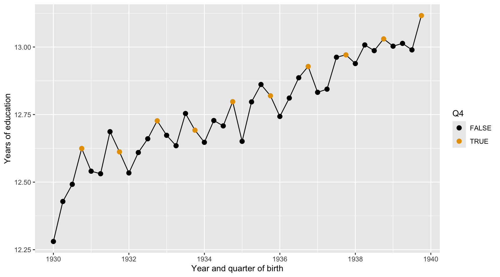

Blank (1)

1. x = YoBQ, y = Educ
2. y = YoBQ, x = Educ
3. x = YoB, y = Educ
4. y = YoB, x = Educ
5. Both a and b
6. Both c and d

Show answer

a

Blank (2)

1. fill
2. color
3. Both a and b

Show answer

b

Blank (3)

1. geom_scatterplot
2. geom_point
3. geom_line
4. geom_smooth
5. geom_histogram
6. geom_boxplot
7. geom_bar
8. geom_col

Show answer

c

Question 38

Here we describe the quarterly trend of the base-10 log of wage per week. Complete the code by filling in the blanks (1)-(3).

ggplot(data = ak91_age, 
       mapping = aes(___(1)___,
                     ___(2)___ = Q4)) +
  ___(3)___ + 
  geom_point(size = 2.5) +
  scale_color_colorblind() +
  labs(x = "Year and quarter of birth",
       y = "Wage per week (in base-10 log)")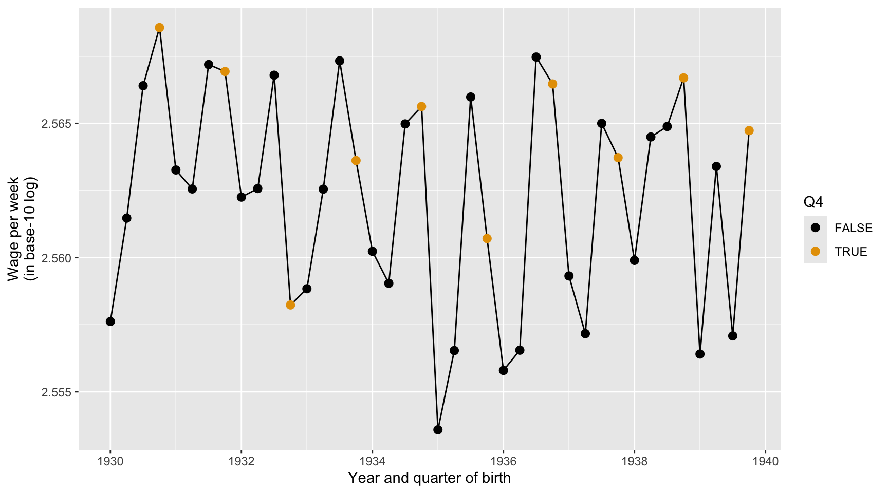

Blank (1)

1. x = YoBQ, y = log(W)
2. y = YoBQ, x = log(W)
3. x = YoBQ, y = log10(W)
4. y = YoBQ, x = log10(W)
5. Both a and c
6. Both b and d

Show answer

c

Blank (2)

1. fill
2. color
3. Both a and b

Show answer

b

Blank (3)

1. geom_scatterplot
2. geom_point
3. geom_line
4. geom_smooth
5. geom_histogram
6. geom_boxplot
7. geom_bar
8. geom_col

Show answer

c

Question 39

Here we describe how the distribution of the base-10 log of wage per week varies by Q4. Complete the code by filling in the blanks (1)-(3).

ggplot(data = ak91_age, 
       mapping = aes(___(1)___,
                     ___(2)___ = Q4)) +
  ___(3)___(show.legend = FALSE) +
  scale_fill_tableau() +
  labs(x = "Wage per week (in base-10 log)",
       y = "Born in the Fourth Quarter?")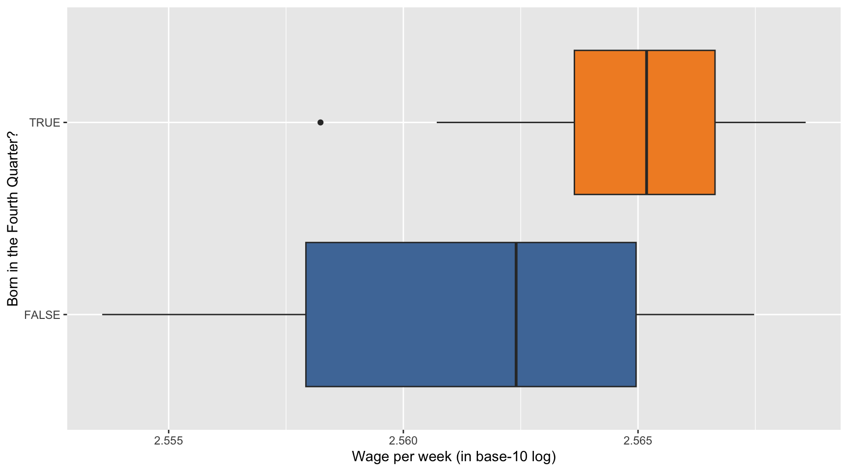

Blank (1)

1. x = YoBQ, y = log(W)
2. y = YoBQ, x = log(W)
3. x = YoBQ, y = log10(W)
4. y = YoBQ, x = log10(W)
5. x = Q4, y = log(W)
6. y = Q4, x = log(W)
7. x = Q4, y = log10(W)
8. y = Q4, x = log10(W)
9. Both a and c
10. Both b and d
11. Both e and g
12. Both f and h

Show answer

h

Blank (2)

1. fill
2. color
3. Both a and b

Show answer

a

Blank (3)

1. geom_scatterplot
2. geom_point
3. geom_line
4. geom_smooth
5. geom_histogram
6. geom_boxplot
7. geom_bar
8. geom_col

Show answer

f

Question 40

Provide a data-driven narrative for the ak91_age data frame, incorporating insights from the visualizations created in Questions 37, 38, and 39.

Show answer

First, years of education increase steadily for men born from 1930 to 1939. Later birth cohorts tend to have more schooling than earlier cohorts, suggesting that educational attainment improved over time.

Second, holding birth year constant, men born in the fourth quarter tend to have slightly more years of education than men born in other quarters. This is consistent with the idea that quarter of birth can be related to schooling because of school-entry and compulsory-schooling rules.

Third, men born in the fourth quarter also appear to have slightly higher weekly wages on average. The boxplot shows that the median wage for the fourth-quarter group is a little higher.

Overall, the figures support the idea behind the Angrist and Krueger setting: quarter of birth is related to education, and education may be related to wages. However, the wage differences by quarter of birth are relatively small and variable.

Questions 41-44

For Questions 41-44, consider the following R packages and the data.frame, health_cust, which contains demographic information about individuals with or without health insurance.

library(tidyverse)
library(skimr)
library(ggthemes)

health_cust <- read_csv(
  'https://bcdanl.github.io/data/custdata_rev.csv'
)

The first 10 observations in the health_cust data frame are displayed below:

custid	sex	is_employed	income	marital_status	housing_type
000006646_03	Male	TRUE	22000	Never married	Homeowner free and clear
000007827_01	Female	NA	23200	Divorced/Separated	Rented
000008359_04	Female	TRUE	21000	Never married	Homeowner with mortgage/loan
000008529_01	Female	NA	37770	Widowed	Homeowner free and clear
000008744_02	Male	TRUE	39000	Divorced/Separated	Rented
000011466_01	Male	NA	11100	Married	Homeowner free and clear
000015018_01	Female	TRUE	25800	Married	Rented
000017314_02	Female	NA	34600	Married	Homeowner free and clear
000017383_04	Female	TRUE	25000	Never married	Homeowner free and clear
000017554_02	Male	TRUE	31200	Married	Homeowner with mortgage/loan

custid	recent_move	num_vehicles	age	state_of_res	gas_usage	health_ins
000006646_03	FALSE	0	24	Alabama	210	FALSE
000007827_01	TRUE	0	82	Alabama	3	FALSE
000008359_04	FALSE	2	31	Alabama	40	FALSE
000008529_01	FALSE	1	93	Alabama	120	FALSE
000008744_02	FALSE	2	67	Alabama	3	FALSE
000011466_01	FALSE	2	76	Alabama	200	FALSE
000015018_01	FALSE	2	26	Alabama	3	TRUE
000017314_02	FALSE	2	73	Alabama	50	FALSE
000017383_04	FALSE	5	27	Alabama	3	FALSE
000017554_02	FALSE	3	54	Alabama	20	FALSE

Description of Variables in health_cust

• custid: ID of customer
• sex: Sex
• is_employed: Employment status
  • NA: Unknown or not applicable
  • TRUE: Employed
  • FALSE: Unemployed
• income: Income (in $)
• marital_status: Marital status
• housing_type: Housing type
• recent_move:
  • TRUE: Recently moved
  • FALSE: Not recently moved
• age: Age
• state_of_res: State of residence (Alabama, Alaska, …, New York, …, Wyoming)
• gas_usage: Gas usage
  • NA: Unknown or not applicable
  • 001: Included in rent or condo fee
  • 002: Included in electricity payment
  • 003: No charge or gas not used
  • 004-999: $4 to $999 (rounded and top-coded)
• health_ins: Health insuarance status
  • TRUE: customer with health insuarance
  • FALSE: customer without health insuarance

The followings are the summary of the health_cust data.frame, including descriptive statistics for each variable.

Data summary

Name	health_cust
Number of rows	73262
Number of columns	12
_______________________
Column type frequency:
character	5
logical	3
numeric	4
________________________
Group variables	None

Variable type: character

skim_variable	n_missing	min	max	empty	n_unique
custid	0	12	12	0	73262
sex	0	4	6	0	2
marital_status	0	7	18	0	4
housing_type	1720	6	28	0	4
state_of_res	0	4	20	0	51

Variable type: logical

skim_variable	n_missing	mean	count
is_employed	25774	0.95	TRU: 45137, FAL: 2351
recent_move	1721	0.13	FAL: 62418, TRU: 9123
health_ins	0	0.10	FAL: 65955, TRU: 7307

Variable type: numeric

skim_variable	n_missing	mean	sd	p0	p25	p50	p75	p100
income	0	41764.15	58113.76	-6900	10700	26200	51700	1257000
num_vehicles	1720	2.07	1.17	0	1	2	3	6
age	0	49.16	18.08	0	34	48	62	120
gas_usage	1720	41.17	63.05	1	3	10	60	570

Question 41

Here we describe how the distribution of health_ins varies by state of residence and employment status using the health_cust data.frame. Complete the code by filling in the blanks (1)-(4).

ggplot(data = health_cust |> filter(!is.na(is_employed)),
       mapping = aes(___(1)___, 
                     fill = ___(2)___)) +
  ___(3)___ +
  ___(4)___(~is_employed) +
  labs(y = "", x= "Proportion") +
  scale_fill_tableau()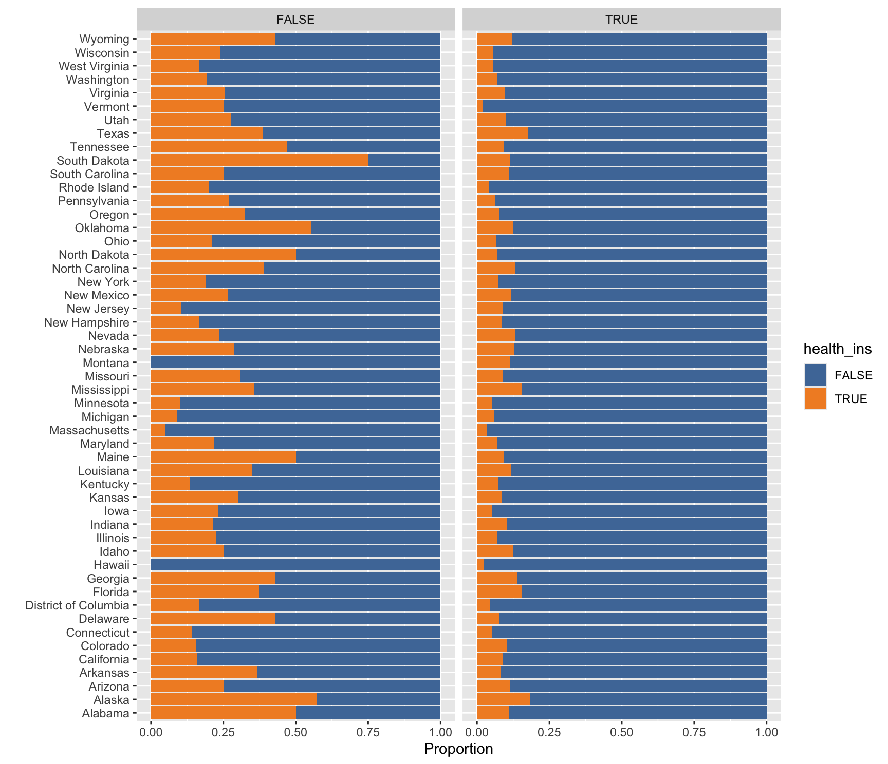

Blank (1)

1. x = health_ins
2. x = state_of_res
3. x = Proportion
4. y = health_ins
5. y = state_of_res
6. y = Proportion

Show answer

e

Blank (2)

1. health_ins
2. state_of_res
3. Proportion

Show answer

a

Blank (3)

1. geom_bar(position = "stack")
2. geom_col(position = "stack")
3. geom_bar(position = "fill")
4. geom_col(position = "fill")
5. geom_bar(position = "dodge")
6. geom_col(position = "dodge")

Show answer

c

Blank (4)

Answer: ________________________________________

Show answer

facet_wrap

Question 42

Here we describe how the distribution of marital_status varies by housing_type using the health_cust data.frame. Complete the code by filling in the blanks (1)-(4).

ggplot(data = health_cust |> filter(!is.na(housing_type)),
       mapping = aes(___(1)___, 
                     ___(2)___)) +
  ___(3)___(show.legend = FALSE) +
  ___(4)___(~housing_type) +
  labs(y = "")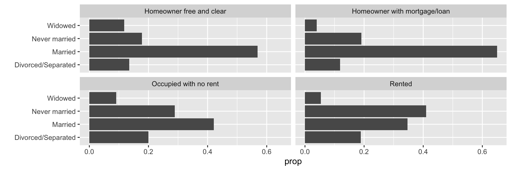

Blank (1)

1. x = marital_status
2. y = marital_status

Show answer

b

Blank (2)

1. x = prop
2. x = prop, group = 1
3. Both a and b
4. y = prop
5. y = prop, group = 1
6. Both d and e
7. x = after_stat(prop)
8. x = after_stat(prop), group = 1
9. Both g and h
10. y = after_stat(prop)
11. y = after_stat(prop), group = 1
12. Both j and k

Show answer

h

Blank (3)

1. geom_bar()
2. geom_col()
3. Both a and b

Show answer

a

Blank (4)

Answer: ________________________________________

Show answer

facet_wrap

Question 43

Here we describe how the relationship between age and income varies by health_ins using the health_cust data.frame. Note that the new geometric object geom_hex() divides the plane into regular hexagons, counts the number of observations in each hexagon, and then maps the number of observations to the hexagon fill.

Complete the code by filling in the blanks (1)-(4).

# Considering 
  # income level between $0 and $250,000
  # age between 20 and 70
ggplot(data = health_cust |> filter(income >= 0 & income <= 2.5*10^5,
                                    age >= 20 & age <= 70),
       mapping = aes(___(1)___)) +
  geom_hex() + # hexbin plot: dividing the plot area into hexagonal bins
  ___(2)___ +
  ___(3)___(~health_ins) +
  scale_fill_viridis_c() # for hexbin color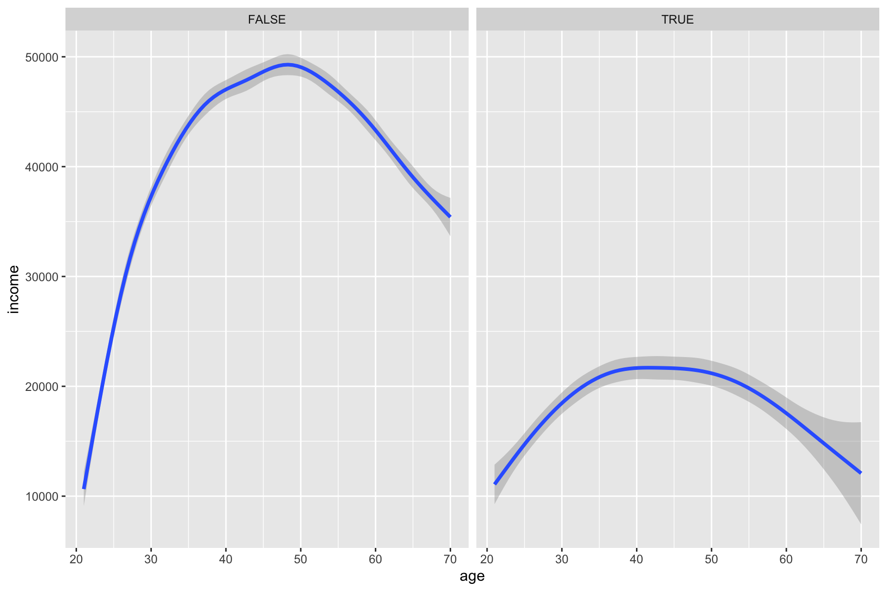

Blank (1)

1. x = income, y = age
2. x = age, y = income

Show answer

b

Blank (2)

1. geom_smooth()
2. geom_smooth(method = "lm")
3. Both a and b

Show answer

a

Blank (3)

Answer: ________________________________________

Show answer

facet_wrap

Question 44

Describe how the overall relationship between age and income varies by health_ins.

Show answer

Overall, both groups show an inverted U-shaped relationship between age and income, but individuals without health insurance tend to have substantially higher incomes and experience a steeper increase in earnings during early and middle adulthood.