Lecture 12

pandas Basics - Reshaping DataFrames; Joining DataFrames; Data Concatenation

Byeong-Hak Choe

bchoe@geneseo.edu

SUNY Geneseo

February 24, 2025

Reshaping DataFrames

Reshaping DataFrames

Tidy DataFrames

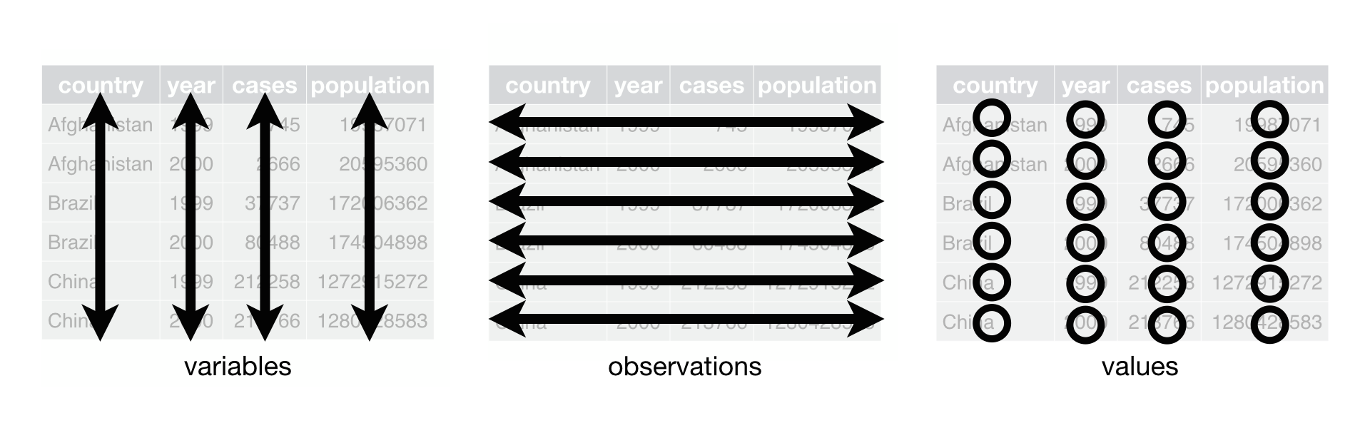
• There are three interrelated rules that make a DataFrame tidy:
  • Each variable is a column; each column is a variable.
  • Each observation is a row; each row is an observation.
  • Each value is a cell; each cell is a single value.

Reshaping DataFrames

• A DataFrame can be given in a format unsuited for the analysis that we would like to perform on it.

  • A DataFrame may have larger structural problems that extend beyond the data.
  • Perhaps the DataFrame stores its values in a format that makes it easy to extract a single row but difficult to aggregate the data.

• Reshaping a DataFrame means manipulating it into a different shape.

• In this section, we will discuss pandas techniques for molding a DataFrame into the shape we desire.

Long vs. Wide DataFrames

• The following DataFrames measure temperatures in two cities over two days.

import pandas as pd
from google.colab import data_table
data_table.enable_dataframe_formatter()

df_wide = pd.DataFrame({
    'Weekday': ['Tuesday', 'Wednesday'],
    'Miami': [80, 83],
    'Rochester': [57, 62],
    'St. Louis': [71, 75]
})

df_long = pd.DataFrame({
    'Weekday': ['Tuesday', 'Wednesday', 'Tuesday', 'Wednesday', 'Tuesday', 'Wednesday'],
    'City': ['Miami', 'Miami', 'Rochester', 'Rochester', 'St. Louis', 'St. Louis'],
    'Temperature': [80, 83, 57, 62, 71, 75]
})

Long vs. Wide DataFrames

• A DataFrame can store its values in wide or long format.
• These names reflect the direction in which the data set expands as we add more values to it.
  • A long DataFrame increases in height.
  • A wide DataFrame increases in width.

Long vs. Wide DataFrames

• The optimal storage format for a DataFrame depends on the insight we are trying to glean from it.
  • We consider making DataFrames longer if one variable is spread across multiple columns.
  • We consider making DataFrames wider if one observation is spread across multiple rows.

Reshaping DataFrames

melt() and pivot()

• melt() makes DataFrame longer.
• pivot() makes DataFrame wider.

Make DataFrame Longer with melt()

df_wide_to_long = (
    df_wide
    .melt()
)

Make DataFrame Longer with melt()

df_wide_to_long = (
    df_wide
    .melt(id_vars = "Weekday")
)

• melt() can take a few parameters:
  • id_vars is a container (string, list, tuple, or array) that represents the variables that will remain as is.
  • id_vars can indicate which column should be the “identifier”.

Make DataFrame Longer with melt()

df_wide_to_long = (
    df_wide
    .melt(id_vars = "Weekday",
          var_name = "City",
          value_name = "Temperature")
)

• melt() can take a few parameters:
  • var_name is a string for the name of the variable whose values are taken from column names in a given wide-form DataFrame.
  • value_name is a string for the name of the variable whose values are taken from the values in a given wide-form DataFrame.

Make DataFrame Wider with pivot()

df_long_to_wide = (
    df_long
    .pivot(index = "Weekday",
           columns = "City",
           values = "Temperature"  
        )
    .reset_index()
    )

• When using pivot(), we need to specify a few parameters:
  • index that takes the column to pivot on;
  • columns that takes the column to be used to make the variable names of the wider DataFrame;
  • values that takes the column that provides the values of the variables in the wider DataFrame.

Reshaping DataFrames

• Let’s consider the following wide-form DataFrame, df, containing information about the number of courses each student took from each department in each year.

dict_data = {"Name": ["Donna", "Donna", "Mike", "Mike"],
             "Department": ["ECON", "DANL", "ECON", "DANL"],
             "2018": [1, 2, 3, 1],
             "2019": [2, 3, 4, 2],
             "2020": [5, 1, 2, 2]}
df = pd.DataFrame(dict_data)

df_longer = df.melt(id_vars=["Name", "Department"], 
                    var_name="Year", 
                    value_name="Number of Courses")

• The pivot() method can also take a list of variable names for the index parameter.

Reshaping DataFrames

• Let’s consider the following wide-form DataFrame, df, containing information about the number of courses each student took from each department in each year.

dict_data = {"Name": ["Donna", "Donna", "Mike", "Mike"],
             "Department": ["ECON", "DANL", "ECON", "DANL"],
             "2022": [1, 2, 3, 1],
             "2023": [2, 3, 4, 2],
             "2024": [5, 1, 2, 2]}
df = pd.DataFrame(dict_data)

df_longer = df.melt(id_vars=["Name", "Department"], 
                    var_name="Year", 
                    value_name="Number of Courses")

Q. How can we use the df_longer to create the wide-form DataFrame, df_wider, which is equivalent to the df?

Reshaping DataFrames

Let’s do Part 1 of Classwork 7!

Joining DataFrames

Joining DataFrames

Relational Data

• Sometimes, one data set is scattered across multiple files.
  • The size of the files can be huge.
  • The data collection process can be scattered across time and space.
  • E.g., DataFrame for county-level data and DataFrame for geographic information, such as longitude and latitude.
• Sometimes we want to combine two or more DataFrames based on common data values in those DataFrames.
  • This task is known in the database world as performing a “join.”
  • We can do this with the merge() method in Pandas.

Joining DataFrames

Relational Data

• The variables that are used to connect each pair of tables are called keys.

Joining DataFrames with merge()

x = pd.DataFrame({
    'key': [1, 2, 3],
    'val_x': ['x1', 'x2', 'x3']
})

y = pd.DataFrame({
    'key': [1, 2, 4],
    'val_y': ['y1', 'y2', 'y3']
})

• The colored column represents the “key” variable.
• The grey column represents the “value” column.

Joining DataFrames with merge()

Inner Join

• An inner join matches pairs of observations whenever their keys are equal:

# the default value for 'how' is 'inner'
# so it doesn't actually need to be specified
merge_inner = pd.merge(x, y, on='key', how='inner')
merge_inner_x = x.merge(y, on='key', how='inner')
merge_inner_x_how = x.merge(y, on='key')

Joining DataFrames with merge()

Left Join

• A left join keeps all observations in x.

merge_left = pd.merge(x, y, on='key', how='left')
merge_left_x = x.merge(y, on='key', how='left')

• The most commonly used join is the left join.

Joining DataFrames with merge()

Right Join

• A right join keeps all observations in y.

merge_right = pd.merge(x, y, on='key', how='right')
merge_right_x = x.merge(y, on='key', how='right')

Joining DataFrames with merge()

Outer (Full) Join

• A full join keeps all observations in x and y.

merge_outer = pd.merge(x, y, on='key', how='outer')
merge_outer_x = x.merge(y, on='key', how='outer')

Joining DataFrames with merge()

Duplicate keys: one-to-many

• One DataFrame has duplicate keys (a one-to-many relationship).

x = pd.DataFrame({
    'key':[1, 2, 2, 3],
    'val_x':['x1', 'x2', 'x3', 'x4']})

y = pd.DataFrame({
    'key':[1, 2],
    'val_y':['y1', 'y2'] })
one_to_many = x.merge(y, on='key', 
                         how='left')

Joining DataFrames with merge()

Duplicate keys: many-to-many

• Both DataFrames have duplicate keys (many-to-many relationship).

x = pd.DataFrame({
  'key':[1, 2, 2, 3],
  'val_x':['x1','x2','x3','x4']})

y = pd.DataFrame({
  'key': [1, 2, 2, 3],
  'val_y': ['y1', 'y2', 'y3', 'y4'] })
many_to_many = x.merge(y, on='key', 
                          how='left')

Joining DataFrames with merge()

Defining the key columns

• If the left and right columns do not have the same name for the key variables, we can use the left_on and right_on parameters instead.

x = pd.DataFrame({
  'key_x': [1, 2, 3],
  'val_x': ['x1', 'x2', 'x3']
})

y = pd.DataFrame({
  'key_y': [1, 2],
  'val_y': ['y1', 'y2'] })

keys_xy = 
  x.merge(y, left_on = 'key_x', 
             right_on = 'key_y', 
             how = 'left')

Joining DataFrames with merge()

Let’s do Part 2 of Classwork 7!

Data Concatenation

Data Concatenation

• Concatenation can be thought of as appending a row or column to our data.
  • This approach is possible if our data was split into parts or if we performed a calculation that we want to append to our existing data set.
• Let’s consider the following example DataFrames:

df1 = pd.read_csv('https://bcdanl.github.io/data/concat_1.csv')
df2 = pd.read_csv('https://bcdanl.github.io/data/concat_2.csv')
df3 = pd.read_csv('https://bcdanl.github.io/data/concat_3.csv')

• We will be working with .index and .columns in this Section.

df1.index
df1.columns

Data Concatenation

Add Rows

• Concatenating the DataFrames on top of each other uses the concat() method.
  • All of the DataFrames to be concatenated are passed in a list.

row_concat = pd.concat([df1, df2, df3])
row_concat

Data Concatenation

Add Rows

• Let’s consider a new Series and concatenate it with df1:

# create a new row of data
new_row_series = pd.Series(['n1', 'n2', 'n3', 'n4'])
new_row_series


# attempt to add the new row to a dataframe
df = pd.concat([df1, new_row_series])
df

• Not only did our code not append the values as a row, but it also created a new column completely misaligned with everything else.
• Why?

Data Concatenation

Add Rows

• To fix the problem, we need turn our Series into a DataFrame.
  • This data frame contains one row of data, and the column names are the ones the data will bind to.

new_row_df = pd.DataFrame(
  # note the double brackets to create a "row" of data
  data =[["n1", "n2", "n3", "n4"]],
  columns =["A", "B", "C", "D"],
)

df = pd.concat([df1, new_row_df])

Data Concatenation

Add Columns

• Concatenating columns is very similar to concatenating rows.
  • The main difference is the axis parameter in the concat() method.
  • The default value of axis is 0 (or axis = "index"), so it will concatenate data in a row-wise fashion.
  • If we pass axis = 1 (or axis = "columns") to the function, it will concatenate data in a column-wise manner.

col_concat = pd.concat([df1, df2, df3], axis = "columns")

Data Concatenation

Add Columns

• We can use ignore_index=True to reset the column indices, so that we do not have duplicated column names.

pd.concat([df1, df2, df3], axis="columns", ignore_index=True)

Concatenate with Different Indices

• What would happen when the row and column indices are not aligned?

• Let’s modify our DataFrames for the next few examples.

# rename the columns of our dataframes
df1.columns = ['A', 'B', 'C', 'D']
df2.columns = ['E', 'F', 'G', 'H']
df3.columns = ['A', 'C', 'F', 'H']

• If we try to concatenate these DataFrames as we did, the DataFrames now do much more than simply stack one on top of the other.

row_concat = pd.concat([df1, df2, df3])

Concatenate with Different Indices

• We can set join = 'inner' to keep only the columns that are shared among the data sets.

pd.concat([df1, df2, df3], join ='inner')

• If we use the DataFrames that have columns in common, only the columns that all of them share will be returned.

pd.concat([df1, df3], join ='inner',  ignore_index =False)

Concatenate with Different Indices

• Let’s modify our DataFrames further.

# re-indexing the rows of our DataFrames
df1.index = [0, 1, 2, 3]
df2.index = [4, 5, 6, 7]
df3.index = [0, 2, 5, 7]

Concatenate with Different Indices

• When we concatenate along axis="columns" (axis=1), the new DataFrames will be added in a column-wise fashion and matched against their respective row indices.

col_concat = pd.concat([df1, df2, df3], axis="columns")

• Just as we did when we concatenated in a row-wise manner, we can choose to keep the results only when there are matching indices by using join="inner".

pd.concat([df1, df3], axis ="columns", join='inner')

Data Concatenation

Let’s do Part 3 of Classwork 7!