Lecture 24
Clutter is Your Enemy!
November 1, 2024
Happy Halloween, everyone! 🎃👻🎃👻🎃👻🎃👻🎃👻🎃👻


Clutter is Your Enemy!
Visualization Principle
Cognitive Load
- Every element added to a page or screen demands cognitive load
- Cognitive load: the mental effort needed to process information
- Extra elements = extra brain power for the audience to process
- Example: Overly complex slides or graphs can overwhelm viewers
- Excessive load can lead to disengagement and confusion
- Goal: a graphic should display as much information as it can, with the lowest possible cognitive strain to the viewer.
Visualization Principle
Why Reduce Clutter?
- Clutter: Visual elements that occupy space but do not improve understanding
- Clutter makes information harder to process and can confuse the viewer
- Strive for clarity: Simplified visuals encourage engagement and improve comprehension
- Less clutter = clearer message, more focused audience
- Tips
- Avoid having the data all skewed to one side or the other of your graph.
- Avoid too many superimposed elements, such as too many curves (>4) in the same graphing space.
Clutter is Your Enemy!

- Which one do you prefer?
Log Transformation: Reducing Clutter in Scatterplots
- Problem: When data points are densely packed, it can obscure insights
- Often due to extreme values or skewed distributions
- Dense clusters of points become visual clutter, hiding patterns
- Solution: Apply a log transformation!
- Reduces clutter: Points become evenly distributed across the plot
- Prevents overlapping data points and enhances readability
- Reduces influence of outliers, clarifying patterns
- Improves interpretability by revealing underlying relationships
- Supports focused, informative data communication without extra elements
- Reduces clutter: Points become evenly distributed across the plot
Log Transformation: Reducing Clutter in Scatterplots
A Little Bit of Math for Logarithm
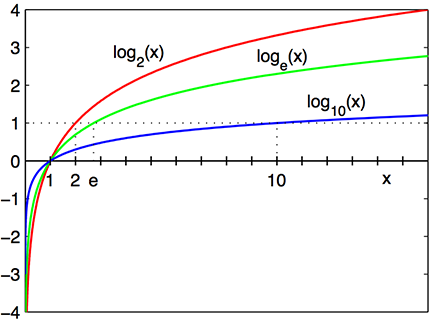
- The logarithm function, \(y = \log_{b}\,(\,x\,)\), looks like ….

Log Transformation: Reducing Clutter in Scatterplots
A Little Bit of Math for Logarithm
\(\log_{10}\,(\,100\,)\): the base \(10\) logarithm of \(100\) is \(2\), because \(10^{2} = 100\)
\(\log_{e}\,(\,x\,)\): the base \(e\) logarithm is called the natural log, where \(e = 2.718\cdots\) is the mathematical constant, the Euler’s number.
\(\log\,(\,x\,)\) or \(\ln\,(\,x\,)\): the natural log of \(x\) .
\(\log_{e}\,(\,7.389\cdots\,)\): the natural log of \(7.389\cdots\) is \(2\), because \(e^{2} = 7.389\cdots\).
In R,
log(x): log ofxwith base e, called natural log.log10(x): log ofxwith base 10.
Log Transformation: Reducing Clutter in Scatterplots
The Use of Logarithm: Wide Range of Skewed Data
- We should consider using a log scale when a variable is heavily skewed.
- It can help visualize both small and large values effectively.


Log Transformation: Reducing Clutter in Scatterplots
The Use of Logarithm: Percentage Change
- Consider using a logarithmic scale when percentage changes are more meaningful than changes in absolute units.
- Percentage changes are widely used in various fields to better interpret relative differences. Examples include:
- Stock prices: Percentage changes reflect the magnitude of gains or losses relative to the initial price.
- Housing prices: Percentage changes show market trends consistently across different neighborhoods or regions.
- GDP growth: Expressed as a percentage to indicate economic performance over time.
- Income levels: A $1,000 increase has a greater impact on a lower-income individual compared to someone with a significantly higher income.
Log Transformation: Reducing Clutter in Scatterplots
The Use of Logarithm: Percentage Change
- For a small change in variable \(x\) from \(x_{0}\) to \(x_{1}\), we have:
\[ \Delta \log(x) = \log(x_{1}) - \log(x_{0}) \approx \frac{x_{1} - x_{0}}{x_{0}} = \frac{\Delta x}{x_{0}}. \]
- This shows that a log transformation effectively represents percentage change!
Visualization Principle
Clutter is Your Enemy!


- One percent increase in GDP per capita is associated with an increase in life expectancy by 0.084 year (30.66 days)!