Lecture 14
Data Preparation and Management with R
September 30, 2024
Joining Relational data.frames with left_join()
Pipe (|>) Operator
tidyversefunctions work well with the pipe,|>, because the first argument of atidyversefunction is adata.frameand the output is adata.frame.- Ctrl + Shift + M for Windows; command + Shift + M for Mac.
- The pipe (
|>) takes the thing on its left and passes it along to the function on its right so thatf(x, y)is equivalent tox |> f(y).- e.g.,
left_join(DATA.FRAME_1, DATA.FRAME_2)is equivalent toDATA.FRAME_1 |> left_join(DATA.FRAME_2).
- The easiest way to pronounce the pipe (
|>) is “then”.- The pipe (
|>) is super useful when we have a chain of data transforming operations to do.
- The pipe (
Pipe (|>) Operator
To use the (native) pipe operator (
|>), we should set the option as follows:- Tools > Global Options > Code from the side menu > Choose “Use native pipe operator, |>”.
Joining Relational data.frames with left_join()

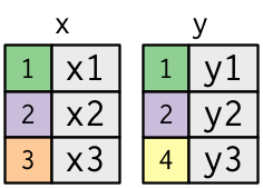
- The colored column represents the “key” variable.
- The grey column represents the “value” column.
Relational Data

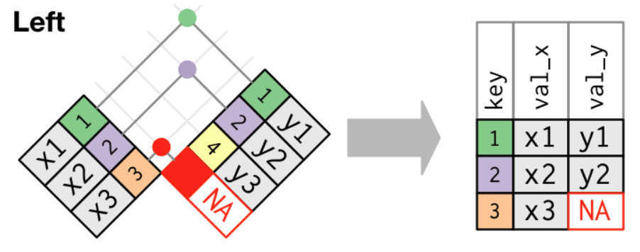
- A left join keeps all observations in
x.- The left join is most commonly used.
- Note:
NAstands for “not available” (i.e., a missing value).
Data Transformation with R tidyverse
Data Transformation
DATA.FRAME |> filter(LOGICAL_CONDITIONS)DATA.FRAME |> arrange(VARIABLES)DATA.FRAME |> select(VARIABLES)DATA.FRAME |> rename(NEW_VARIABLE = EXISTING_VARIABLE)The subsequent arguments describe what to do with the data.frame, mostly using the variable names.
The result is a data.frame.
Filter observations with filter()
Filter observations with filter()
jan1 <- flights |>
  filter(month == 1, day == 1)

dec25 <- flights |>
  filter(month == 12, day == 25)

class(flights$month == 1)filter()allows us to subset observations based on the value of logical conditions, which are eitherTRUEorFALSE.
Filter observations with filter()
Logicals and Conditions
- Logical variables have either
TRUEorFALSEvalue. - Conditions are expressions that evaluate as
logical. - What logical operations do is combining logical conditions, which returns a logical value when executed.
Filter observations with filter()
Logical Operations
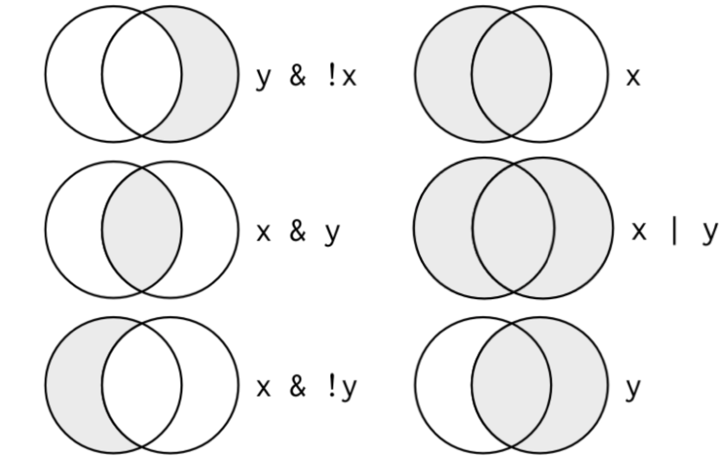
xis the left-hand circle,yis the right-hand circle, and the shaded region show which parts each operator selects.
