Lecture 8
R Basics
September 13, 2024
R Basics
Descriptive Statistics

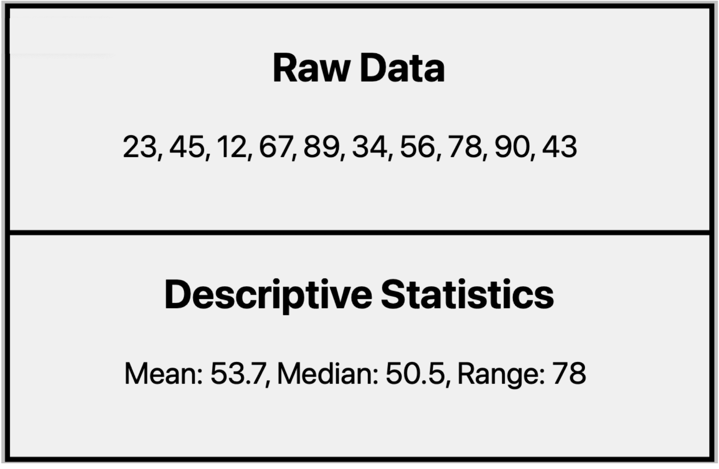
Descriptive statistics condense data into manageable summaries, making it easier to understand key characteristics of the data.
- They help reveal patterns, trends, and relationships within the data that might not be immediately apparent from raw numbers.
Descriptive Statistics
- Data quality assessment:
- Descriptive statistics can highlight potential issues in data quality, such as outliers or unexpected distributions, prompting further investigation.
- Foundation for further analysis:
- Descriptive statistics often serve as a starting point for more advanced statistical analyses and predictive modeling.
- Data visualization enhancement:
- Descriptive statistics often form the basis for effective data visualizations, making complex data more accessible and understandable.
Descriptive Statistics
Measures of Central Tendency
- Measures of centrality are used to describe the central or typical value in a given vector.
- They represent the “center” or most representative value of a data set.
- To describe this centrality, several statistical measures are commonly used:
- Mean: The arithmetic average of all values in the data set.
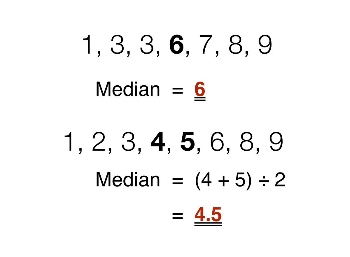
- Median: The middle value when the data set is ordered from least to greatest.
- Mode: The most frequently occurring value in the data set.
Measures of Central Tendency
Mean
\[ \overline{x} = \frac{x_{1} + x_{2} + \cdots + x_{N}}{N} \]
- The arithmetic mean (or simply mean or average) is the sum of all the values divided by the number of observations in the data set.
mean()calculates the mean of the values in a vector.- For a given vector \(x\), if we happen to have \(N\) observations \((x_{1}, x_{2}, \cdots , x_{N})\), we can write the arithmetic mean of the data sample as above.
Measures of Central Tendency
Median


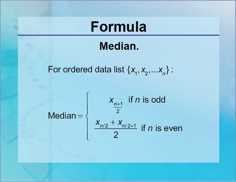
- The median is the measure of center value in a given vector.
median()calculates the median of the values in a vector.
Measures of Central Tendency
Mode
The mode is the value(s) that occurs most frequently in a given vector.
Mode is useful, although it is often not a very good representation of centrality.
The R package,
modest, provides themfw(x)function that calculate the mode of values in vectorx.
Descriptive Statistics
Measures of Dispersion
- Measures of dispersion are used to describe the degree of variation in a given vector.
- They are a representation of the numerical spread of a given data set.
- To describe this dispersion, a number of statistical measures are developed
- Range
- Variance
- Standard deviation
- Quartile
Measures of Dispersion
Range
\[ (\text{range of x}) \,=\, (\text{maximum value in x}) \,-\, (\text{minimum value in x}) \]
- The range is the difference between the largest and the smallest values in a given vector.
max(x)returns the maximum value of the values in a given vector \(x\).min(x)returns the minimum value of the values in a given vector \(x\).
Measures of Dispersion
Variance
\[ \overline{s}^{2} = \frac{(x_{1}-\overline{x})^{2} + (x_{2}-\overline{x})^{2} + \cdots + (x_{N}-\overline{x})^{2}}{N-1}\;\, \]
- The variance is used to calculate the deviation of all data points in a given vector from the mean.
- The larger the variance, the more the data are spread out from the mean and the more variability one can observe in the data sample.
- To prevent the offsetting of negative and positive differences, the variance takes into account the square of the distances from the mean.
var(x)calculates the variance of the values in a vector \(x\).
Measures of Dispersion
Standard Deviation
\[ \overline{s} = \sqrt{ \left( \frac{(x_{1}-\overline{x})^{2} + (x_{2}-\overline{x})^{2} + \cdots + (x_{N}-\overline{x})^{2}}{N-1}\;\, \right) } \]
- The standard deviation (SD)—the square root of the variance—is also a measure of the spread of values within a given vector.
sd(x)calculates the standard deviation of the values in a vector \(x\)- SD helps us understand how representative the mean is of the data.
- A low SD suggests that the mean is a good summary, while a high SD suggests greater variability around the mean.
Measures of Dispersion
Quartiles
quantile(x)
quantile(x, 0) # the minimum
quantile(x, 0.25) # the 1st quartile
quantile(x, 0.5) # the 2nd quartile
quantile(x, 0.75) # the 3rd quartile
quantile(x, 1) # the maximum- A quartile is a quarter of the number of data points in a given vector.
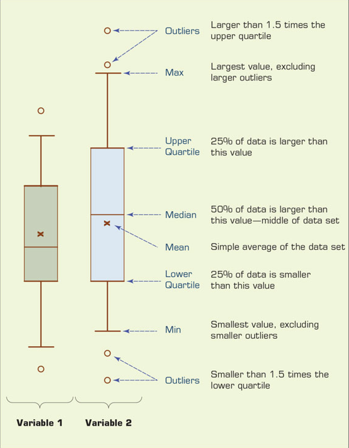
- Quartiles are determined by first sorting the values and then splitting the sorted values into four disjoint smaller data sets.
- Quartiles are a useful measure of dispersion because they are much less affected by outliers or a skewness in the data set than the equivalent measures in the whole data set.
Measures of Dispersion
Interquartile Range

- An interquartile range describes the difference between the third quartile (Q3) and the first quartile (Q1), telling us about the range of the middle half of the scores in the distribution.
- The quartile-driven descriptive measures (both centrality and dispersion) are best explained with a popular plot called a box plot.
R Basics
CSV file
A CSV (comma-separated values) file is a text file in which values are separated by commas.
CSV files are most commonly encountered in spreadsheets and databases.
Example
https://bcdanl.github.io/data/tvshows.csv
R Basics
Absolute Pathnames
- Complete path from the root directory to the target file or directory.
- Independent of the working directory.
getwd()returns the pathname of the working directory.- The working directory for a Posit Cloud project is
/cloud/project/
- Example of absolute pathnames for
custdata_rev.csv- Mac:
/Users/user/documents/data/custdata_rev.csv
- Windows:
C:\\Users\\user\\Documents\\data\\custdata_rev.csv
- Mac:
R Basics
Relative Pathnames
Path relative to the working directory.
Example:
- Absolute pathname for
custdata_rev.csvis/Users/user/documents/data/custdata_rev.csv. - Suppose the working directory is
/Users/user/documents/. - Then, the relative pathname for
custdata_rev.csvisdada/custdata_rev.csv.
- Absolute pathname for
When using the Posit Cloud project, we can use a relative path to read a file.
R Basics
Working with Data from Files
- We use the
read_csv()function to read a comma-separated values (CSV) file.
Download the CSV file,
custdata_rev.csvfrom the Class Files module in our Brightspace.Create a sub-directory,
data, by clicking “New Folder” in the Files Pane in Posit Cloud.Upload the
custdata_rev.csvfile to the sub-directorydata.Provide the relative pathname for the file,
custdata_rev.csv, to theread_csv()function.
View()displays the data in a simple spreadsheet-like grid.
R Basics
Examining data.frames
dim()shows how many rows and columns are in the data fordata.frame.nrow()andncol()shows the number of rows and columns fordata.framerespectively.skimr::skim()refers to theskim()function from theskimrpackage.- This provides a more comprehensive summary.
- It’s a more user-friendly alternative to functions like base-R’s
summary(), offering both numerical and categorical summaries.