Lecture 7

Big Data and the Modern Data Infrastructure

Byeong-Hak Choe

bchoe@geneseo.edu

SUNY Geneseo

October 15, 2025

A Simple Taxonomy of Data

Structured Data vs. Unstructured Data

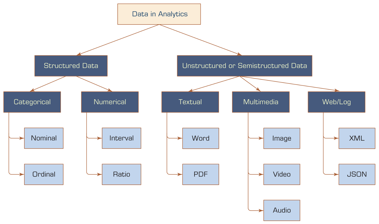
• Data comes in various formats.
  • Structured data: Has a predefined format, fits into traditional databases.
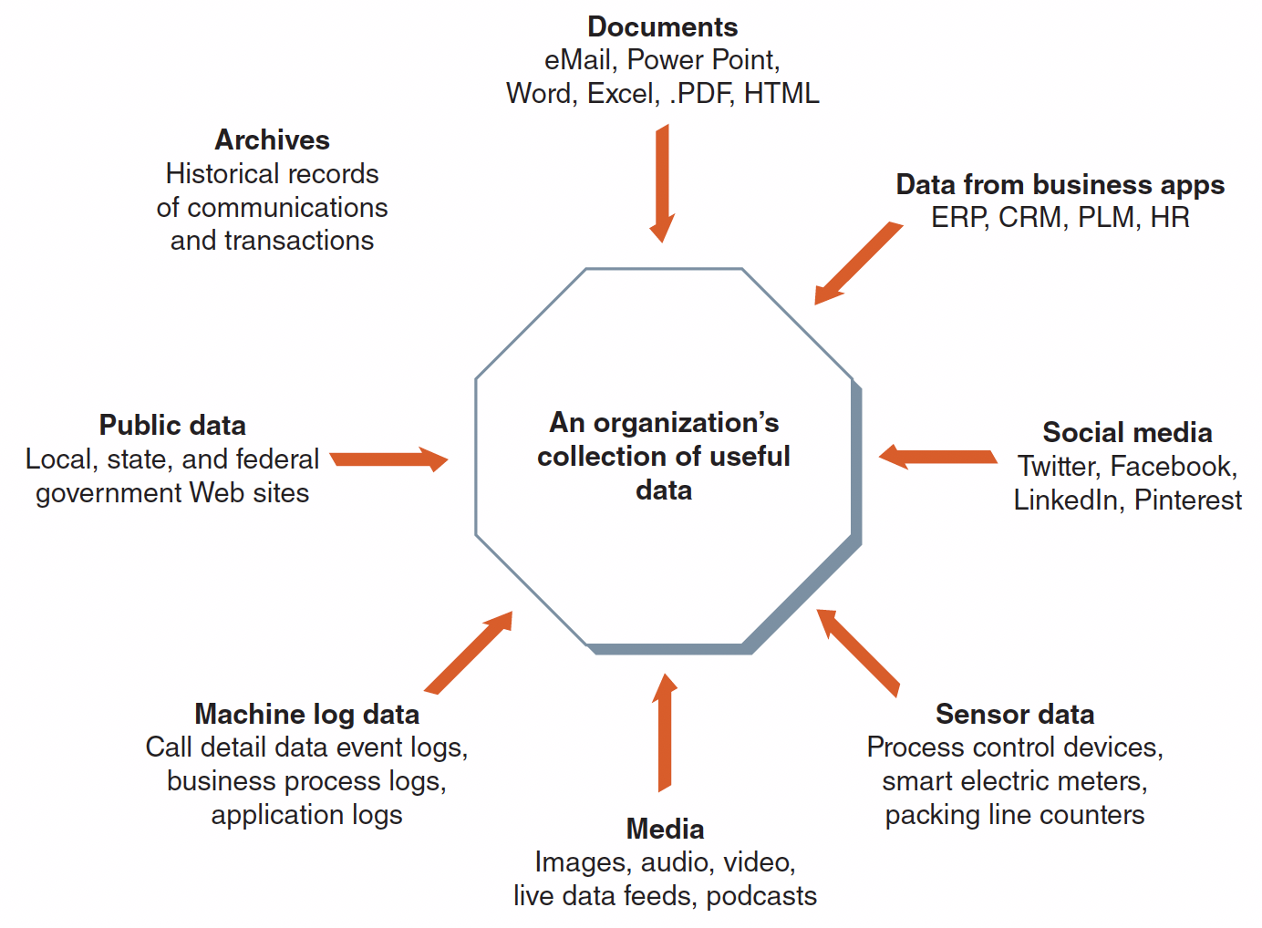
  • Unstructured data: Not organized in a predefined manner, comes from sources like documents, social media, emails, photos, videos, etc.

Data Types Overview

• Categorical Data: Data that can be divided into distinct categories based on some qualitative attribute.
  • Nominal Data
  • Ordinal Data

• Numeric Data: Data that represents measurable quantities and can be subjected to mathematical algebra.
  • Interval Data
  • Ratio Data

Categorical Data - Nominal

ID	Animal
1	Dog
2	Cat
3	Bird

• Nominal Data: Categorical data where the categories have no intrinsic order or ranking.
• No Order: Categories are simply different; there is no logical sequence.
• Examples:
  • Colors: Red, Blue, Green
  • Types of Animals: Dog, Cat, Bird

Categorical Data - Ordinal

ID	Education Level
1	Bachelor’s
2	Master’s
3	PhD

• Ordinal Data: Categorical data where the categories have a meaningful order or ranking.

• Order Matters: Categories can be ranked or ordered, but the differences between categories are not necessarily uniform.

• Examples:

  • Education Levels: High School, Bachelor’s, Master’s, PhD
  • Customer Satisfaction: Poor, Fair, Good, Excellent

Numeric Data - Interval

ID	Temperature (°F)
1	70
2	80
3	90

• Interval Data: Numeric data where the differences between values are meaningful, but there is no true zero point.

• Meaningful Intervals: The difference between values is consistent.

• No True Zero: Zero does not indicate the absence of the quantity.

• Examples:

  • Temperature (°F): Zero degrees does not mean no temperature.
  • Time of Day in a 12-Hour Clock: Differences are meaningful, but there is no absolute zero.

Numeric Data - Ratio

ID	Height (cm)	Weight (kg)
1	160	55
2	175	70
3	170	65

• Ratio Data: Numeric data with a true zero point, allowing for a full range of mathematical operations.

• Meaningful Ratios: Comparisons like twice as much or half as much are valid.

• True Zero: Zero indicates the absence of the quantity.

• Examples:

  • Height in Centimeters: Zero means no height.
  • Weight in Kilograms: Zero means no weight.

Classwork: Taxonomy of Data

Try it out → Classwork 7: Taxonomy of Data

Databases

What Is a Database?

• A database (DB) is a structured collection of data stored electronically.
• A Database Management System (DBMS) is software that helps us:
  • Store data (safely and efficiently)
  • Query data (like filter(), select())
  • Update data while keeping everything consistent and valid
• Examples of DBMS:
  • PostgreSQL / MySQL (used by websites and companies)
  • Google BigQuery, Snowflake (large-scale analysis on cloud system)
  • Excel / Google Sheets → basic storage only — not a full DBMS

Note

• SQL stands for Structured Query Language, and a query simply means asking the data for something — such as filtering rows, selecting columns, or combining information.

ETL: 📥 Extract ➜ 🔧 Transform ➜ 💾 Load

• ETL is the data preparation workflow used in analytics.

ETL Step	Meaning in Data Workflow	Example in a Database Context
Extract	Retrieve raw data from an external source	Importing a CSV, Google Sheet, app response, or web data into a temporary table
Transform	Clean, reshape, and structure the data	Filtering rows, selecting fields, and joining tables
Load	Store the cleaned data for analysis	Writing the final structured table into a database as the analysis-ready dataset

• It makes raw data usable by making it clean, consistent, and connected before analysis begins.

📥 ETL — Extract Stage

• Goal: Collect raw data from external sources
  (Google Sheets, CSV/Excel files, survey tools, web exports, or app submissions).

• Quick Validation Check:

  • ✅ Column names match expected schema
    
  • ✅ Numeric fields contain numbers only (no symbols/text)

• Storage at this stage:

  • Raw data is stored in a temporary DB area (like Google Sheets or CSV)
    
  • ⚠️ This is not yet the official DB — just a collection point

🔧 ETL — Transform Stage

• Goal: Convert raw data into a clean, consistent, analysis-ready format

• In DANL 101 using R (tidyverse):

  • filter() → keep valid observations
  • select() → keep relevant variables
  • *_join() → combine multiple tables/data.frames

• Storage at this stage:

  • Cleaning happens in memory, not yet in the final database
    
  • The Google Sheet + R behave like a database + DBMS system, with tidyverse acting as the query engine

💾 ETL — Load Stage

• Goal: Store the clean, final dataset as the official analysis table

• Storage at this stage:

  • The cleaned data is written to a database area (this becomes the official dataset for analysis)

• In DANL 101 using R (tidyverse):

  • The final data.frame functions as our primary analysis dataset, used for:
    • 📊 Summaries — descriptive statistics and numeric insights
      
    • 📈 Visualizations — plots, charts, and dashboard elements
      
    • 🎯 Storytelling & Analysis — interpreting and communicating insights

• Try it out → Classwork 8: Databases — Social Media Analytics.

Relational Data Thinking

• During the Transform step in ETL, our data becomes:
  • Clean, structured in tables, and organized with a shared key column
• At this point, we start thinking like database analysts:
  • Each table holds one type of data
  • A key column links tables together
• In real-world analytics, data rarely lives in a single big file.
  • Example: one table stores student social media activity
    • Another table stores platform reference information
• To analyze properly, we connect these tables using a key.
  • In R tidyverse: left_join()
  • In database language: a join operation

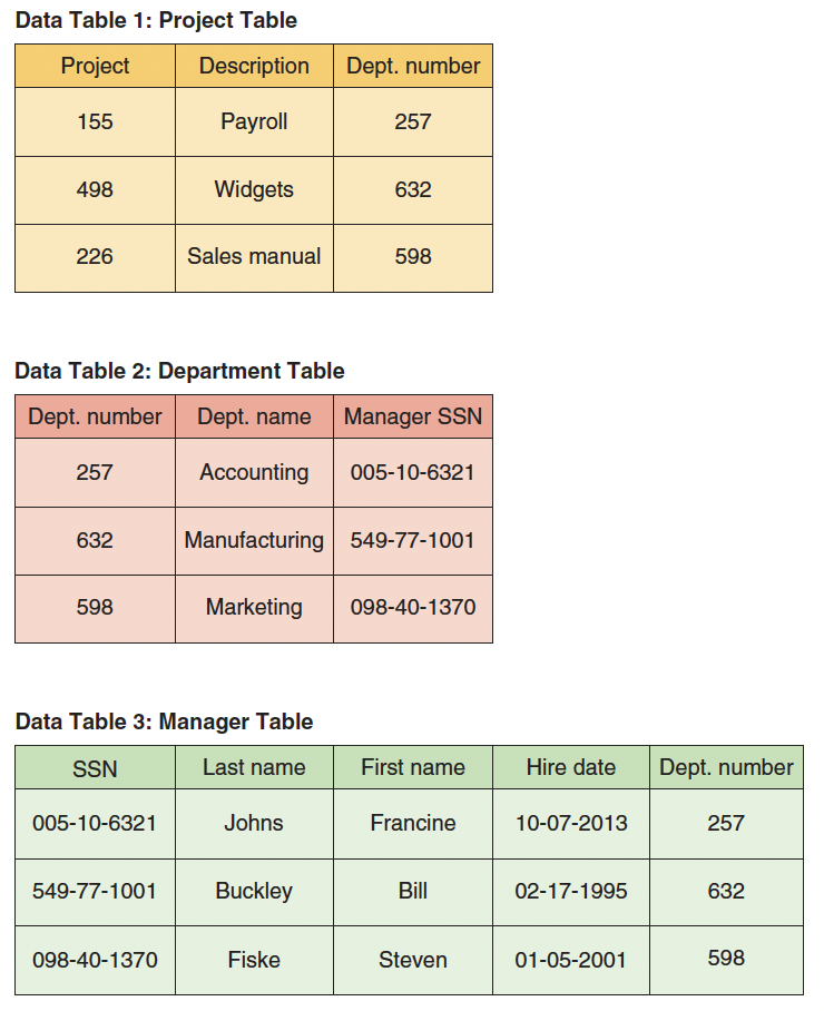
Relational Databases

• When multiple tables are linked by keys, this structure is called a relational database

tab_project <- 
  read_csv("https://bcdanl.github.io/data/rdb-project_table.csv")
tab_department <- 
  read_csv("https://bcdanl.github.io/data/rdb-department_table.csv")
tab_manager <- 
  read_csv("https://bcdanl.github.io/data/rdb-manager_table.csv")

• A relational database organizes data into multiple related tables, called relations.
• Each table stores data about one type of entity (e.g., projects, departments, managers).

Relational Database Characteristics

1. Data is stored in a data.frame (or table).
2. Each row = an observation (or record).
3. Each column = a variable (or attribute or field).
4. Each table has a key — a column that uniquely identifies each row.
5. Keys allow us to link tables together.
6. We use queries (like filter(), select(), left_join()) to retrieve and combine data.

Relational Tables and Keys

x <- data.frame(
    key = c(1, 2, 3),
    val_x = c('x1', 'x2', 'x3')
)

y <- data.frame(
    key = c(1, 2, 4),
    val_y = c('y1', 'y2', 'y3')
)

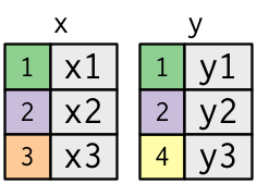
• The colored column represents the “key” variable (key).
• The grey column represents the “value” variable (val_x, val_y).

Joining Tables with left_join()

x |>
  left_join(y)

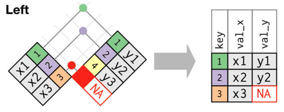
• A left join keeps all rows from x and adds matching information from y.
• Among the different join types, left_join() is the most commonly used join.
  • It does not lose information from your main data.frame (x) and simply attaches extra information (y) when it exists.
• Try it out → Classwork 9: ETL Process in R.

Big Data

What Is Big Data?

• Big data and analytics are key components shaping the future across industries.

• Refers to enormous, complex datasets that traditional tools can’t efficiently manage.

• Characterized by the Five V’s:

  1. Volume — amount of data
     
  2. Velocity — speed of data generation
     
  3. Value — usefulness of data
     
  4. Veracity — trustworthiness of data
     
  5. Variety — diversity of data types

1️⃣ Volume

Unit	Symbol	Value
Kilobyte	kB	10³
Megabyte	MB	10⁶
Gigabyte	GB	10⁹
Terabyte	TB	10¹²
Petabyte	PB	10¹⁵
Exabyte	EB	10¹⁸
Zettabyte	ZB	10²¹
Yottabyte	YB	10²⁴
Brontobyte*	BB	10²⁷
Gegobyte*	GeB	10³⁰

*Less commonly used or proposed extensions.

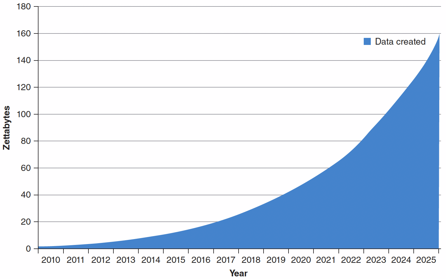
Growth of the Global Datasphere

• In 2017, the digital universe contained 16.1 zettabytes of data.
  
• Expected to grow to 163 zettabytes by 2025.
  

2️⃣ Velocity

• Refers to the rate at which new data is created and processed.
  
• Estimated at 402.74 million terabytes per day (≈181 zettabytes per year).
  
• Around 90% of the world’s data has been generated in just the past two years.

3️⃣ Value

• Represents the worth of data in driving better decisions.
  
• Highlights the need to extract actionable insights quickly.
  
• Large datasets enable discovery of patterns and anomalies not visible in small samples.

4️⃣ Veracity

• Measures data quality and reliability.
  
• Involves accuracy, completeness, and timeliness.
  
• Determines whether data can be trusted for decision-making.

5️⃣ Variety

Technologies for Big Data Management

Why We Need New Technologies

• Big data exceeds what traditional tools can store or analyze.
• Limitations:
  • Legacy databases struggle with volume and speed.
  • Hardware can’t scale efficiently.
• Solutions:
  • Modern frameworks and architectures like Data Warehouses enable:
    • Massive storage
      
    • Fast queries
      
    • Integration across platforms

Schema in Big Data Management

• A schema is the blueprint or structure that defines how data is organized in a database.
  
• It specifies:
  • What fields exist (e.g., name, age, income)
  • What type each field is (e.g., character, number, date)
  • How tables relate to each other
• In other words, a schema tells the system how to read and interpret data consistently.

Data Warehouses

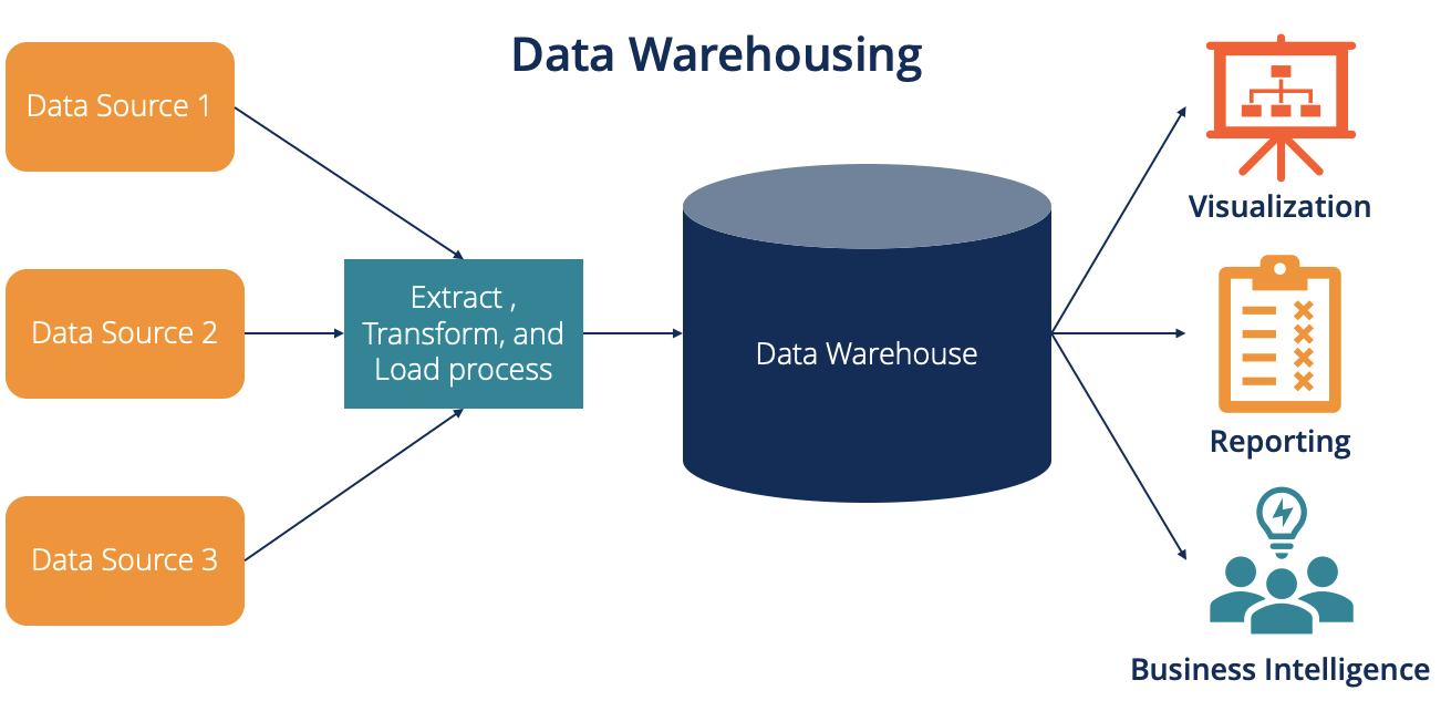
• Definition: Central repository integrating data from multiple sources.
• Purpose: Enables comprehensive analysis and decision-making.

Key Characteristics of Data Warehouses

Characteristic	Description
Large	Stores billions of records and petabytes of data
Multiple Sources	Integrates internal and external data via ETL
Historical	Often includes 5+ years of archived data
Cross-Organizational	Accessible across departments for data-driven strategy
Supports Analysis & Reporting	Enables drill-downs and trend detection
Schema-Based	Data fits a predefined structure before being stored for efficient querying and analysis

Understanding Schema

• Definition: Data is structured and validated before it enters the system.
  • The schema is predefined, specifying tables, fields, and data types.
    
• Advantages:
  • Ensures data consistency, accuracy, and performance
    
  • Ideal for reporting, dashboards, and business intelligence
    
  • Simplifies regulatory compliance and governance
    
• Example:
  • Before inserting sales data, ETL scripts ensure each record matches the schema — e.g.,
    • store_id (integer), sales (numeric)
      
  • Once loaded, users can query with confidence

Walmart: A Pioneer in Data Warehousing

• Early adopter of data-driven supply chain optimization
  

• Collects transaction data from 11,000+ stores and 25,000 suppliers
  

• Uses real-time analytics to optimize pricing, inventory, and customer experience

• In 1992, launched the first commercial data warehouse to exceed 1 TB
  

• In 2025, processes data at a rate of 2.5 petabytes per hour