Lecture 6
R Basics
September 9, 2024
R Basics
R Basics
Data Types
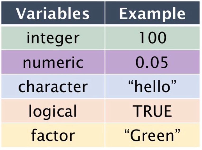
- Logical:
TRUEorFALSE. - Numeric: Numbers with decimals
- Integer: Integers
- Character: Text strings
- Factor: Categorical values.
- Each possible value of a factor is known as a level.
R Basics
Data Containers
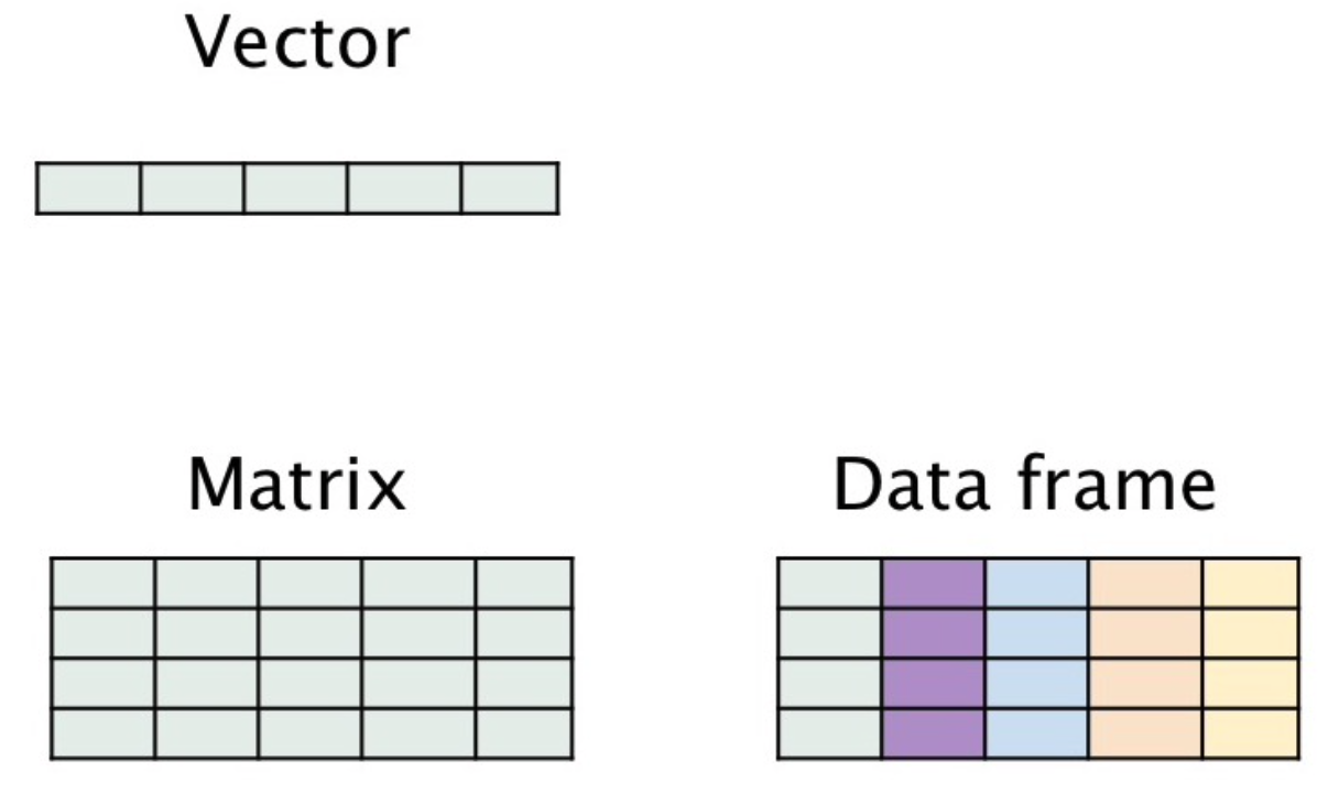
- vector: 1D collection of variables of the same type
- data.frame: 2D collection of variables of multiple types
- A data.frame is a collection of vectors.
R Basics
Data Types
Sometimes we need to explicitly cast a value from one type to another.
- We can do this using built-in functions like
as.character(),as.integer(),as.numeric(), andas.factor().
- We can do this using built-in functions like
R Basics
Data Types
- Strings are known as
characterin R. - Use the double quotes (
") or single quotes (') to wrap around the string- Most IDE, including RStudio, automatically provides a pair of quotes when typing just one quote.
favorite.integer <- as.integer(2)
class(favorite.integer)

favorite.numeric <- as.numeric(8.8)
class(favorite.numeric)- Numbers have different classes.
- The most common two are integer and numeric. Integers are whole numbers.
class(TRUE)
class(FALSE)
favorite.numeric == 8.8
favorite.numeric == 9.9
class(favorite.numeric == 8.8)- We use the
==to test for equality in R
a <- 1:10  # colon operator
b <- c("3", 4, 5)
beers <- c("BUD LIGHT", "BUSCH LIGHT", "COORS LIGHT",
           "MILLER LITE", "NATURAL LIGHT")
class(a)
class(b)
class(beers)
We can create one-dimensional data structures called “vectors”.
c(...): Returns a vector that is constructed from one or more arguments, with the order of the vector elements corresponding to the order of the arguments.
Factors store categorical data.
Under the hood, factors are actually integers that have a string label attached to each unique integer.
- For example, if we have a long list of
Male/Femalelabels for each of our patients, this will be stored a “column” of zeros and ones by R.
- For example, if we have a long list of
R Basics
Workflow: Quotation marks, parentheses, and +
- Quotation marks and parentheses must always come in a pair.
- If not, Console Pane will show you the continuation character
+:
- If not, Console Pane will show you the continuation character
- The
+tells you that R is waiting for more input; it doesn’t think you’re done yet.
R Basics
Functions
A function can take any number and type of input parameters and return any number and type of output results.
R ships a vast number of built-in functions.
R also allows a user to define a new function.
We will mostly use built-in functions.
R Basics
Functions, Arguments, and Parameters
library(tidyverse)

# The function `str_c()`, provided by `tidyverse`, concatenates characters.
str_c("Data", "Analytics")
str_c("Data", "Analytics", sep = "!")
We invoke a function by entering its name and a pair of opening and closing parentheses.
Much as a cooking recipe can accept ingredients, a function invocation can accept inputs called arguments.
We pass arguments sequentially inside the parentheses (, separated by commas).
A parameter is a name given to an expected function argument.
A default argument is a fallback value that R passes to a parameter if the function invocation does not explicitly provide one.
R Basics
Arithmetic Operations and Mathematical Functions
All of the basic operators with parentheses we see in mathematics are available to use.
R can be used for a wide range of mathematical calculations.
- R has many built-in mathematical functions that facilitate calculations and data analysis.
abs(x): the absolute value \(|x|\)sqrt(x): the square root \(\sqrt{x}\)exp(x): the exponential value \(e^x\), where \(e = 2.718...\)log(x): the natural logarithm \(\log_{e}(x)\), or simply \(\log(x)\)
R Basics
Vectorized Operations
- Vectorized operations mean applying a function to every element of a vector without explicitly writing a loop.
- This is possible because most functions in R are vectorized, meaning they are designed to operate on vectors element-wise.
- Vectorized operations are a powerful feature of R, enabling efficient and concise code for data analysis and manipulation.
Measures of Central Tendency
- Measures of centrality are used to describe the central or typical value in a given vector.
- They represent the “center” or most representative value of a data set.
- To describe this centrality, several statistical measures are commonly used:
- Mean: The arithmetic average of all values in the data set.
- Median: The middle value when the data set is ordered from least to greatest.
- Mode: The most frequently occurring value in the data set.
Measures of Central Tendency
Mean
\[ \overline{x} = \frac{x_{1} + x_{2} + \cdots + x_{N}}{N} \]
- The arithmetic mean (or simply mean or average) is the sum of all the values divided by the number of observations in the data set.
mean()calculates the mean of the values in a vector.- For a given vector \(x\), if we happen to have \(N\) observations \((x_{1}, x_{2}, \cdots , x_{N})\), we can write the arithmetic mean of the data sample as above.
Measures of Central Tendency
Median
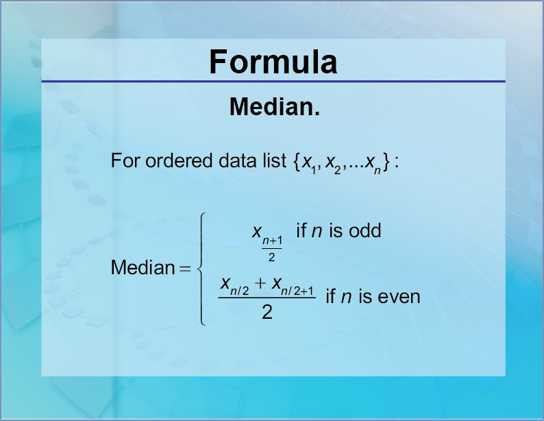
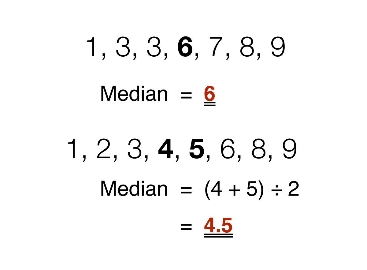
- The median is the measure of center value in a given vector.
median()calculates the median of the values in a vector.
Measures of Central Tendency
Mode
The mode is the value(s) that occurs most frequently in a given vector.
Mode is useful, although it is often not a very good representation of centrality.
The R package,
modest, provides themfw(x)function that calculate the mode of values in vectorx.
Measures of Dispersion
- Measures of dispersion are used to describe the degree of variation in a given vector.
- They are a representation of the numerical spread of a given data set.
- To describe this dispersion, a number of statistical measures are developed
- Range
- Variance
- Standard deviation
- Quartile
Measures of Dispersion
Range
\[ (\text{range of x}) \,=\, (\text{maximum value in x}) \,-\, (\text{minimum value in x}) \]
- The range is the difference between the largest and the smallest values in a given vector.
max(x)returns the maximum value of the values in a given vector \(x\).min(x)returns the minimum value of the values in a given vector \(x\).
Measures of Dispersion
Variance
\[ \overline{s}^{2} = \frac{(x_{1}-\overline{x})^{2} + (x_{2}-\overline{x})^{2} + \cdots + (x_{N}-\overline{x})^{2}}{N-1}\;\, \]
- The variance is used to calculate the deviation of all data points in a given vector from the mean.
- The larger the variance, the more the data are spread out from the mean and the more variability one can observe in the data sample.
- To prevent the offsetting of negative and positive differences, the variance takes into account the square of the distances from the mean.
var(x)calculates the variance of the values in a vector \(x\).
Measures of Dispersion
Standard Deviation
\[ \overline{s} = \sqrt{ \left( \frac{(x_{1}-\overline{x})^{2} + (x_{2}-\overline{x})^{2} + \cdots + (x_{N}-\overline{x})^{2}}{N-1}\;\, \right) } \]
- The standard deviation (SD)—the square root of the variance—is also a measure of the spread of values within a given vector.
sd(x)calculates the standard deviation of the values in a vector \(x\)- SD helps us understand how representative the mean is of the data.
- A low SD suggests that the mean is a good summary, while a high SD suggests greater variability around the mean.
Measures of Dispersion
Quartiles
quantile(x)
quantile(x, 0) # the minimum
quantile(x, 0.25) # the 1st quartile
quantile(x, 0.5) # the 2nd quartile
quantile(x, 0.75) # the 3rd quartile
quantile(x, 1) # the maximum- A quartile is a quarter of the number of data points in a given vector.
- Quartiles are determined by first sorting the values and then splitting the sorted values into four disjoint smaller data sets.
- Quartiles are a useful measure of dispersion because they are much less affected by outliers or a skewness in the data set than the equivalent measures in the whole data set.
Measures of Dispersion
Interquartile Range
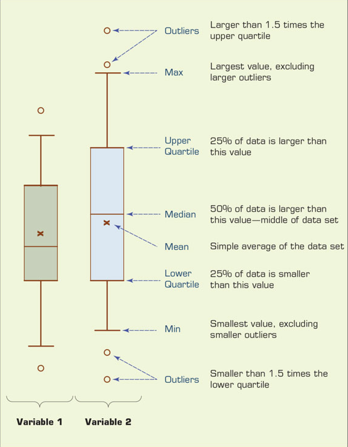
- An interquartile range describes the difference between the third quartile (Q3) and the first quartile (Q1), telling us about the range of the middle half of the scores in the distribution.
- The quartile-driven descriptive measures (both centrality and dispersion) are best explained with a popular plot called a box plot.
R Basics
Absolute vs. Relative Pathnames
Complete path from the root directory to the target file or directory.
Independent of the current working directory.
Example
- Mac:
/Users/user/documents/data/car_data.csv
- Windows:
C:\\Users\\user\\Documents\\data\\car_data.csv
- Mac:
- Path relative to the working directory.
- Relative path changes based on the working directory.
- Example:
- Absolute pathname for
car_data.csvis/Users/user/documents/data/car_data.csv. - Suppose the current directory is
/Users/user/documents/. - Then, the relative pathname for
car_data.csvisdada/car_data.csv.
- Absolute pathname for
- For the Posit Cloud project, we can use a relative path.
- The current working directory in is
/cloud/project/
- The current working directory in is
R Basics
Working with Data from Files
- We use the
read_csv()function to read a comma-separated values (CSV) file.
Download the CSV file,
car_data.csvfrom the Class Files module in our Brightspace.Create a sub-directory,
data, by clicking “New Folder” in the Files Pane in Posit Cloud.Upload the
car_data.csvfile to the sub-directorydata.Provide the relative pathname for the file,
car_data.csv, to theread_csv()function.
View()/view()displays the data in a simple spreadsheet-like grid.
R Basics
Examining data.frames
dim()shows how many rows and columns are in the data fordata.frame.nrow()andncol()shows the number of rows and columns fordata.framerespectively.skimr::skim()provides a more detailed summary.skimris the R package that provides the functionskim().
R Basics
Reading data.frames from an URL
- We can import the CSV file from the web.
R Basics
Tidy data.frame: Variables, Observations, and Values

There are three rules which make a
data.frametidy:- Each variable must have its own column.
- Each observation must have its own row.
- Each value must have its own cell.
:::
–> –> –> –>