Lecture 5
Reading and Transforming Data with R
September 29, 2026
📂 Reading a Data Table as a data.frame
📄 A CSV file is a plain-text table
- A CSV (comma-separated values) file is a plain text file where each value is separated by a comma.
- The first line usually gives the column names.
- Each later line supplies one row of values.
- The commas separate columns.
- CSV files are widely used for storing data from spreadsheets and databases.
- Example
📍 An absolute pathname gives a file’s full location
- An absolute pathname tells the computer the exact location of a file, starting from the very top folder of your computer.
- It does not depend on R’s working directory, but it changes if the file is moved or renamed.
| Computer | Example of an absolute pathname |
|---|---|
| Mac | /Users/USERNAME/Downloads/custdata_rev.csv |
| Windows | C:\Users\USERNAME\Downloads\custdata_rev.csv |
Windows displays the pathname with backslashes (\). When entering it in R, use forward slashes (/) instead:
- R treats a single backslash (
\) as a special character inside quotation marks.
🧭 A relative pathname starts at R’s working directory
The working directory is the folder R uses as its starting point. Run getwd() in the Console to see it.
| Role | Example |
|---|---|
| Given: working directory | /cloud/project |
| Given: CSV file’s full location | /cloud/project/data/custdata_rev.csv |
| Result: relative pathname | data/custdata_rev.csv |
📥 Read a downloaded CSV into R
- Download
custdata_rev.csvfrom the Class Files module in Brightspace.- The file will usually be saved in your computer’s Downloads folder.
- Do not open this file in a spreadsheet app (e.g., Excel or Numbers).
- In Posit Cloud, create a subfolder named data (Files Pane → + Folder).
- Click the data folder, then upload the
custdata_rev.csvfile into it.- At the top of the Files Pane, click Upload to choose and add your file.
- Read the file using a relative pathname:
🧪 Classwork 5: Absolute Pathnames
Find the downloaded file
Copy its absolute pathname
Paste it into a text editor
🌐 A CSV can also be read from a web address
- We can load a CSV file directly from the web into R.
🔎 Getting to Know a data.frame
🔎 Inspect the size and contents of custdata
dim()shows both the number of rows and columns.
nrow()andncol()give the row count and column count separately.
summary()gives a quick overview, whileskimr::skim()provides a more detailed, user-friendly summary of variables across all data types.
💲 operator extracts a column as a vector
The $ operator extracts a column from a data.frame as a vector.
🧹 Tidy data gives each value a clear place
In this example, one observation is one customer’s spending in one month.
| Customer | Month | Spending |
|---|---|---|
| Ana | January | 42 |
| Ana | February | 38 |
| Bo | January | 55 |
- Each variable has its own column.
- Each observation has its own row.
- Each value has its own cell.
👥 Observations in data.frame
- Rows in a data.frame represent individual units or entities for which data is collected.
- Examples:
- Student Information: Each row = one student
- Employee Information: Each row = one employee
- Daily S&P 500 Index Data: Each row = one trading day
- Household Survey Data: Each row = one household
- Student Information: Each row = one student
🏷️ Variables in data.frame
- Columns in a data.frame represent attributes or characteristics measured across multiple observations.
- Examples:
- Student Data:
Name,Age,Grade,Major
- Employee Data:
EmployeeID,Name,Age,Department
- Customer Data:
CustomerID,Name,Age,Income,HousingType
- Student Data:
Note
- In a data.frame, a variable is a column of data.
- In general programming, a variable is the name of an object.
🔄 Data Transformation with dplyr
🛠️ dplyr changes a data.frame in useful ways

dplyris a core tidyverse package for data manipulation — tasks like filtering, sorting, selecting, and renaming.
| Function | What changes? |
|---|---|
filter(DF, LOGICAL_CONDITIONS) |
Keep rows that meet a condition |
arrange(DF, VARIABLES) |
Sort rows |
distinct(DF, VARIABLES) |
Keep unique rows or combinations |
select(DF, VARIABLES) |
Select or remove columns |
rename(DF, NEW_NAME = CURRENT_NAME) |
Rename a column name |
dplyrfunctions take a data.frame as a first argument.- They return a data.frame as output.
🔗 The pipe connects steps from left to right
- The pipe operator (
|>or%>%) passes the result on its left into the function on its right- It makes code easier to read by connecting steps in order.
- How it works:
f(x, y)is the same asx |> f(y).
- Example with a data frame
DF:filter(DF, logical_condition)
- is the same as
DF |> filter(logical_condition)
- You can read the pipe as “then”:
- Example: Start with
DF, then keep rows wherelogical_conditionisTRUE.
- Example: Start with
🔗 The pipe works well with dplyr verbs
- Common
dplyrfunctions with the pipe operator:DF |> filter(LOGICAL_CONDITIONS)
DF |> arrange(VARIABLES)
DF |> distinct(VARIABLES)
DF |> select(VARIABLES)
DF |> rename(NEW_NAME = CURRENT_NAME)
- Why this works so well:
dplyrfunctions usually take a data.frame as the first argument.
- They return a data.frame as output.
- This allows you to chain together multiple steps naturally:
- Example: Start with data, then filter, then arrange
\(\qquad\quad\;\;\)DF |> filter(...) |> arrange(...)
- Example: Start with data, then filter, then arrange
☁️ Insert the pipe in RStudio or Posit Cloud
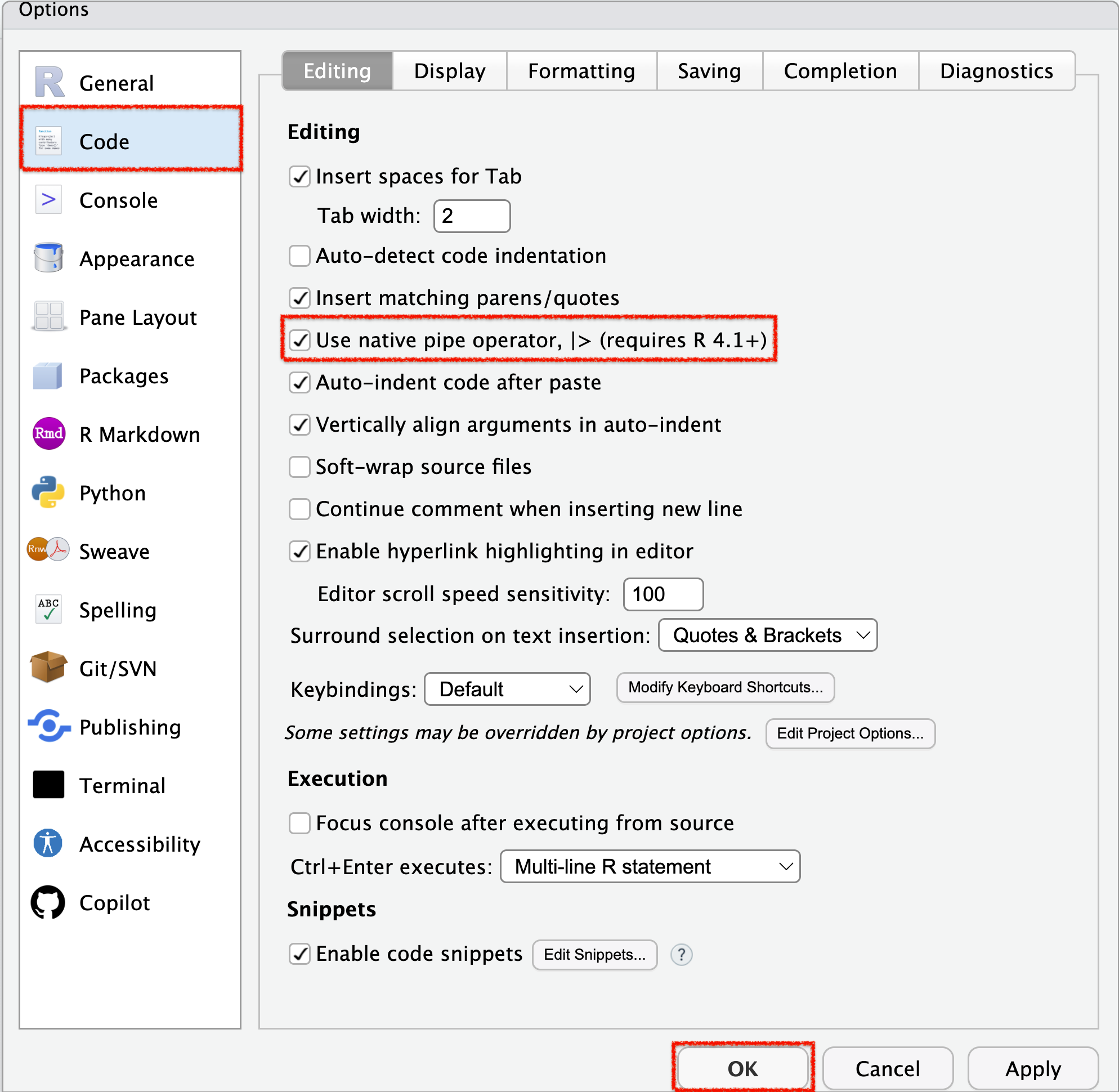
- To enable the native pipe operator (
|>) in RStudio:- Go to Tools > Global Options > Code (side menu).
- Under Pipe operator, choose Use native pipe operator (
|>).
- Go to Tools > Global Options > Code (side menu).
- Keyboard shortcut for inserting a pipe:
- Windows: Ctrl + Shift + M
- Mac: Cmd + Shift + M
- Windows: Ctrl + Shift + M
🎯 Filter observations with filter()
🔢 One small table for our filtering examples
| Row | num |
chr |
|---|---|---|
| 1 | 8 | A |
| 2 | 9 | C |
| 3 | 10 | B |
| 4 | 11 | A |
We will use this df on the next slides.
⚖️ Mathematical comparisons produce TRUE or FALSE
| Condition | Meaning |
|---|---|
V1 == V2 |
Is V1 equal to V2? |
V1 != V2 |
Is V1 not equal to V2? |
V1 > V2 |
Is V1 greater than V2? |
V1 >= V2 |
Is V1 greater than or equal to V2? |
V1 < V2 |
Is V1 less than V2? |
V1 <= V2 |
Is V1 less than or equal to V2? |
- Here, both
V1andV2are variables, and the comparisons are applied element-wise (vectorized).
- For logical conditions using inequalities, we focus on cases where
V1andV2areintegerornumeric.
filter() keeps only the rows where the condition is TRUE
🔣 Combine conditions with logical operators — AND, OR, NOT
- Here, both
xandyarelogicalconditions/variables.
What logical operations (
&,|,!) do is combining logical variables/conditions, returning alogicalvariable when executed.&requires both conditions.|requires at least one condition.!reverses a condition.
🧠 Venn diagram visualizes logical operations
xandyare logical conditions.- If
xisTRUE, it highlights the left circle.
- If
yisTRUE, it highlights the right circle.
- If
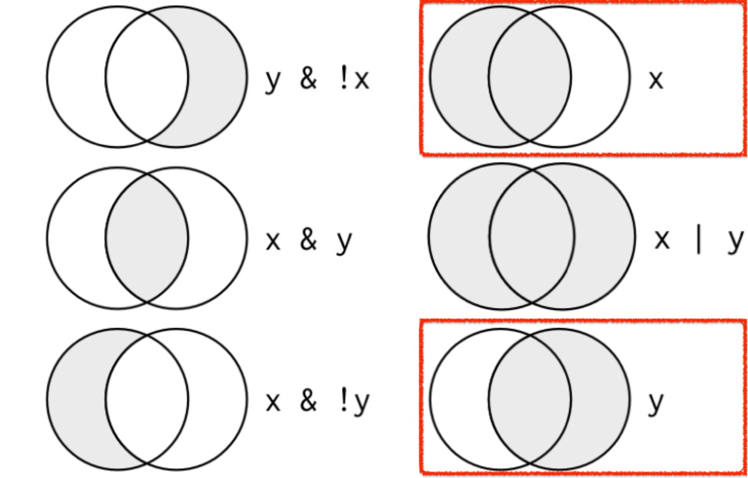
- The shaded regions show which parts each logical operator selects.
& or a comma keeps rows that meet both conditions
- In
filter(), separating conditions with a comma is equivalent to combining them with the&operator.
& can combine conditions on different columns
| keeps rows that meet at least one condition
✈️ Apply the same conditions to flights
The nycflights13 package supplies the flights data frame.
Each condition checks the values in its column, one row at a time.
❓ NA means a value is missing or unknown
NA(not available) represents a missing or unknown value in R.
- In most calculations, if one value is unknown, the result will also be unknown (
NA).
🧮 na.rm = TRUE removes missing values for calculation
- Without
na.rm = TRUE, both functions returnNAfor this vector.
na.rm = TRUEremoves missing values for the calculation.
- Here, R uses only non-missing values,
1and3, for calculation. The original data stay unchanged.
🆚 Comparing Missing Values
- Suppose
v1is Mary’s age (unknown) andv2is John’s age (unknown). - Can we say they are the same age?
- Since both values are missing, R cannot know — so the result is also
NA.
🔎 Checking for Missing Values with is.na()
- Use
is.na()to test whether a value is missing (NA).
- In
filter(), you can:- Use
is.na()to keep observations with missing values. - Use
!is.na()to remove observations with missing values.
- Use
↕️ Arrange Observations with arrange()
⬆️ arrange() sorts whole observations
arrange()sorts out observations.- Missing values appear at the end.
- When you provide multiple variables,
arrange()sorts by the first variable, and then uses the next variable(s) to break ties.
⬇️ desc() reverses the sorting direction
- Use
desc(VARIABLE)to sort in descending order.- For numeric variables, you can also use a leading minus sign.
🔢 Each extra variable in arrange() breaks ties in the one before it
- If we provide more than one variable name, each additional variable will be used to break ties in the values of preceding variables.
🆔 Find All Unique Observations with distinct()
🧹 distinct() removes repeated rows
distinct()removes duplicate observations.- By default, it checks all variables to find unique observations.
🧩 distinct() can check selected columns
- You can pass one or more variables to
distinct().- This returns unique combinations of just those variables (while ignoring the rest).
🧪 Classwork 6: Data Transformation - Rows
filter()
arrange()
distinct()
🎯 Select Variables with select()
📌 select() keeps or removes variables
It’s not uncommon to get datasets with hundreds or thousands of variables.
select()allows us to narrow in on the variables we’re actually interested in.We can select variables by their names.
- With
select(-VARIABLES), we can remove variables.
🏷️ rename() changes a variable name
rename()can be used to rename variables:DF |> rename(NEW_NAME = CURRENT_NAME)
🔄 Put the transformation steps together
- Read the result:
- January flights with a known departure delay
- ordered from the largest delay down
- selecting only three variables
- renaming
dep_delayto the clearer namedeparture_delay
- Check yourself: Which function changed the observations, which changed their order, and which changed the variables?
🧪 Classwork 7: Data Transformation - Columns
select()
rename()