Lecture 5

R Basics

Byeong-Hak Choe

bchoe@geneseo.edu

SUNY Geneseo

September 17, 2025

Posit Cloud & R Packages

Posit Cloud

Posit Cloud (formerly RStudio Cloud) is a web service that delivers a browser-based experience similar to RStudio, the standard IDE for the R language.
For our course, we use Posit Cloud for the R programming component.
- If you want to install R and RStudio on your laptop, you use my office hours.

🚀 Getting Started with Posit Cloud

Click Log In at the top-right corner.
Choose the Sign Up tab from the menu bar.
Create your account using one of the following:
- Google account, or
- Your geneseo.edu or personal email
After logging in, go to New Project → New RStudio Project.
Create a new R script:
- Click the + icon (top-left), or
- Click to File → New File → R script from the menu bar, or
- Use the shortcut:
  - Command + Shift + N (Mac)
  - Ctrl + Shift + N (Windows)

Posit Cloud Environment

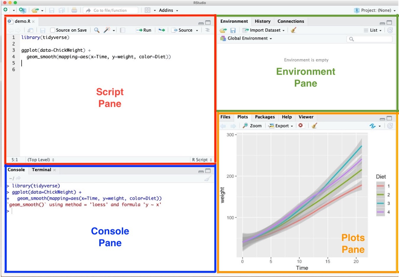
Script Pane is where you write and save R commands in a script file.
- An R script is simply a plain text file containing R code.
- Posit Cloud (RStudio Cloud) automatically color-codes your code to make it easier to read.

Try typing a <- 1 in the Script Pane.
- With the cursor ( ┃ ) on the same line, run the code using:
  - Ctrl + Enter (Windows)
  - Command + Enter (Mac)

Posit Cloud Environment

Console Pane allows you to interact directly with the R interpreter and type commands where R will immediately execute them.

Posit Cloud Environment

Environment Pane shows everything you have created in R so far.
- For example, if you make a variable or a data frame, it will appear here.
- Think of it like a workspace where R keeps track of all the things you’re working on.

Posit Cloud Environment

Plots Pane contains any graphics that you generate from your R code.

📦 R Packages

R packages are collections of ready-made tools for R.
- A package usually includes functions (pre-written commands), data sets, and sometimes extra code to make your work easier.
Many packages are already built into R, and thousands more can be installed from the internet (like downloading apps on your phone).
Why use packages?
- They save time—you don’t need to write everything from scratch.
- They give you access to powerful tools for data analysis, visualization, and more.
Examples:
- readr → for reading data files quickly
- dplyr → for cleaning and transforming data
- ggplot2 → for making beautiful graphs and charts

🌐 `tidyverse`

The tidyverse is a collection of R packages built for data analytics.
- They share a common design philosophy, grammar, and data structures.
Popular packages in the tidyverse include:
- readr → data reading
- dplyr → data transformation
- ggplot2 → data visualization

📦 Installing R Packages with `install.packages("packageName")`

install.packages("tidyverse")

Use the base R function install.packages("packageName") to install new packages.
Example: to install the tidyverse, type and run the command above in the R Console.
While installing, you may see a pop-up question (e.g., about creating a personal library).
- It’s usually safe to answer “No” if you’re unsure.
While running the above codes, you may encounter the pop-up question, and you can answer “No”

📂 Loading R Packages with `library(packageName)`

library(tidyverse)
mpg

After installation, use library(packageName) to load a package into your R session.
Example: running library(tidyverse) loads all the R packages in the tidyverse, including readr, dplyr, and ggplot2.
Once loaded, you can use their functions and datasets.
For instance, mpg is a built-in dataset from ggplot2, which is part of the tidyverse.

Workflow for R packages: Install → Load → Use

Install (once)

install.packages("tidyverse")

Load (At the top of every new R script, load the package:)

library(tidyverse)

Use (functions & datasets)

df <- read_csv("https://bcdanl.github.io/data/spotify_all.csv")

read_csv() function comes from the readr package, which is part of the tidyverse.

Note

🔑 Tip: In Posit Cloud, you need to install a package once per project.
After that, just load it whenever you start a new R script.

Workflow: Naming and File Management

Always save your R script for each class session.
- Go to File → Save (or Save As…), or
- Click the 💾 save icon.
✅ Recommended file naming style (no spaces):
- Example: danl-101-2024-0917.R
Tips for naming files:
- ❌ Avoid spaces in file names.
- ✅ Use lowercase letters and hyphens (-) / underscores (_)

Workflow: Code and comment style

The two main principles for coding and managing data are:
- Make things easier for your future self.
- Don’t trust your future self.
The # mark is R’s comment character.
- In R scripts (*.R files), # indicates that the rest of the line is to be ignored.
- Write comments before the line that you want the comment to apply to.

Workflow: Shortcuts in Posit Cloud

Windows
- Alt + - adds an assignment operator (<-)
- Ctrl + Enter runs a current line of code
- Ctrl + Shift + C makes a comment (- #)
- Ctrl + Shift + R makes a section (- # Section - - - -)

Mac
- option + - adds an assignment operator (<-)
- command + return runs a current line of code
- command + shift + C makes a comment (- #)
- command + shift + R makes a section (- # Section - - - -)

Workflow: Shortcuts in Posit Cloud

Ctrl (command for Mac Users) + Z undoes the previous action.
Ctrl (command for Mac Users) + Shift + Z redoes when undo is executed.

Workflow: Shortcuts in Posit Cloud

Ctrl (command for Mac Users) + F is useful when finding a phrase (and replace the phrase) in the RScript.

Workflow: Auto-completion

libr

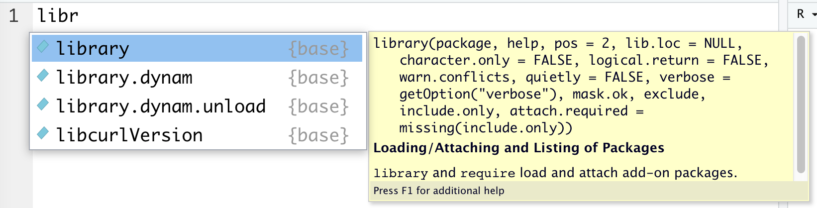
Auto-completion of command is useful.
- Type libr in the RScript in RStudio and wait for a second.

Workflow: STOP icon

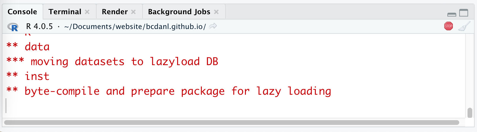
When the code is running, RStudio shows the STOP icon ( 🛑 ) at the top right corner in the Console Pane.
- Do not click it unless if you want to stop running the code.

Posit Cloud Options Setting

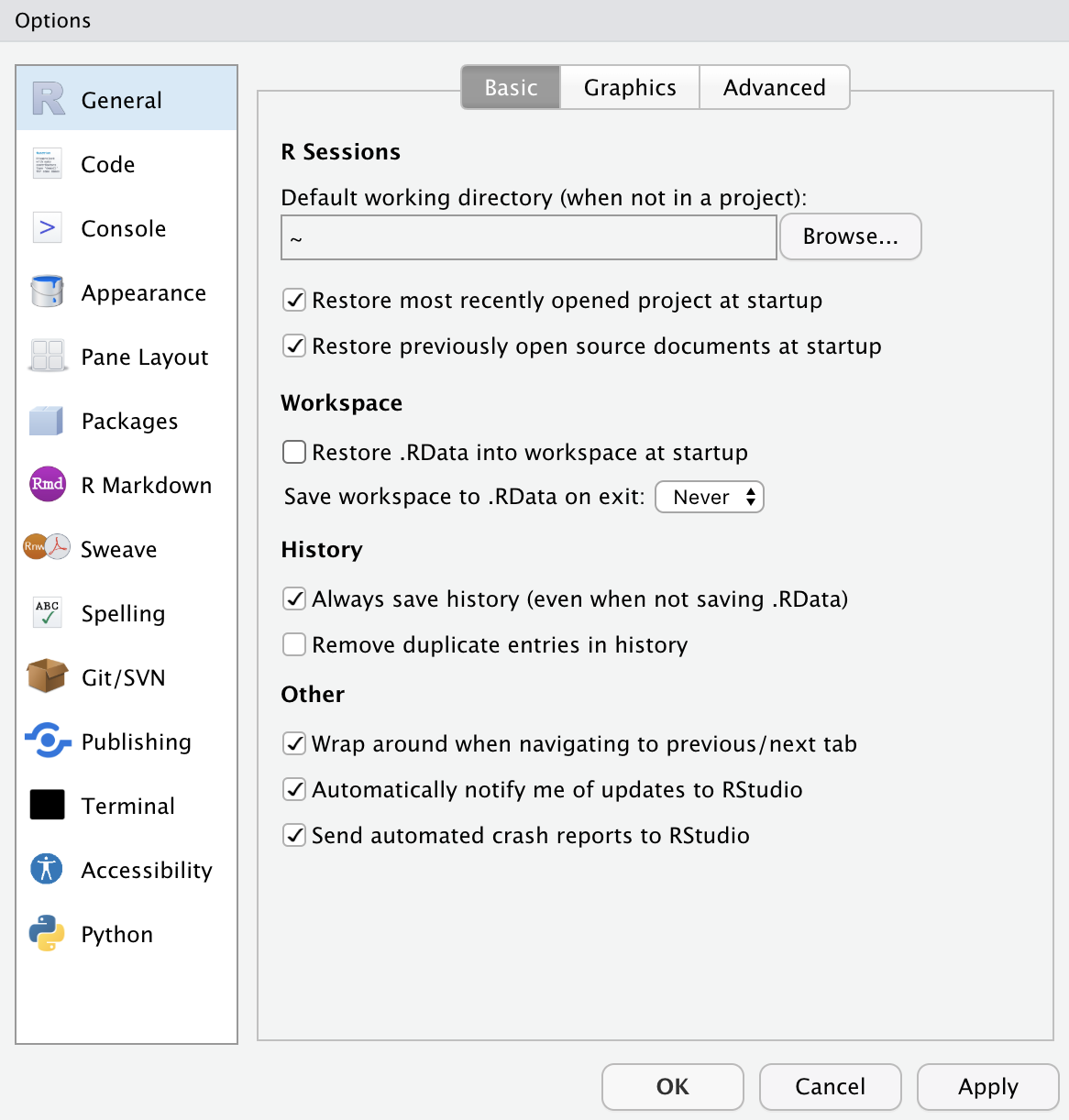
This option menu is found by menus as follows:
- Tools $>$ Global Options
Check the boxes as in the left.
Choose the option Never for Save workspace to .RData on exit:

R Programming Basics

Values, Variables, and Data Types

A value is datum (literal) such as a number or text.
There are different types of values:
- 352.3 is known as a float or double;
- 22 is an integer;
- “Hello World!” is a string.

Values, Variables, and Data Types

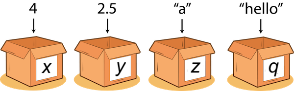
a <- 10    # The most popular assignment operator in R is `<-`.
a

A variable is a name that refers to a value.
- We can think of a variable as a box that has a value, or multiple values, packed inside it.
A variable is just a name!
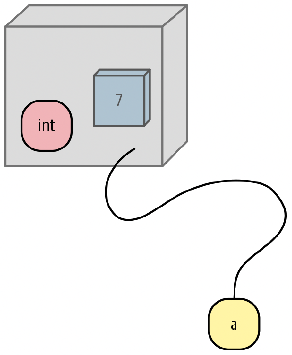
Sometimes you will hear variables referred to as objects. m
Everything that is not a literal value, such as 10, is an object.

Assignment

x <- 2
x < - 3

What is going on here?
The shortcut for the assignment <- is:
- Windows: Alt + -
- Mac: option + -

Assignment

x <- 2
y <- x + 12

In programming code, everything on the right side needs to have a value.
- The right side can be a literal value, or a variable that has already been assigned a value, or a combination.
When R reads y <- x + 12, it does the following:
1. Sees the <- in the middle.
2. Knows that this is an assignment.
3. Calculates the right side (gets the value of the object referred to by x and adds it to 12).
4. Assigns the result to the left-side variable, y.

Data Types

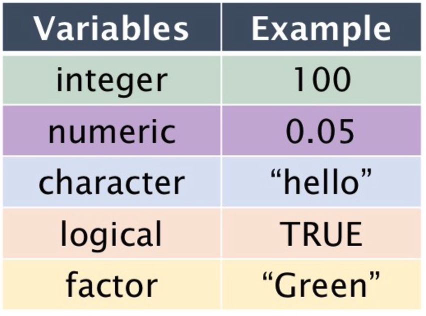
Logical: TRUE or FALSE.
Numeric: Numbers with decimals
Integer: Integers
Character: Text strings
Factor: Categorical values.
- Each possible value of a factor is known as a level.

Data Containers

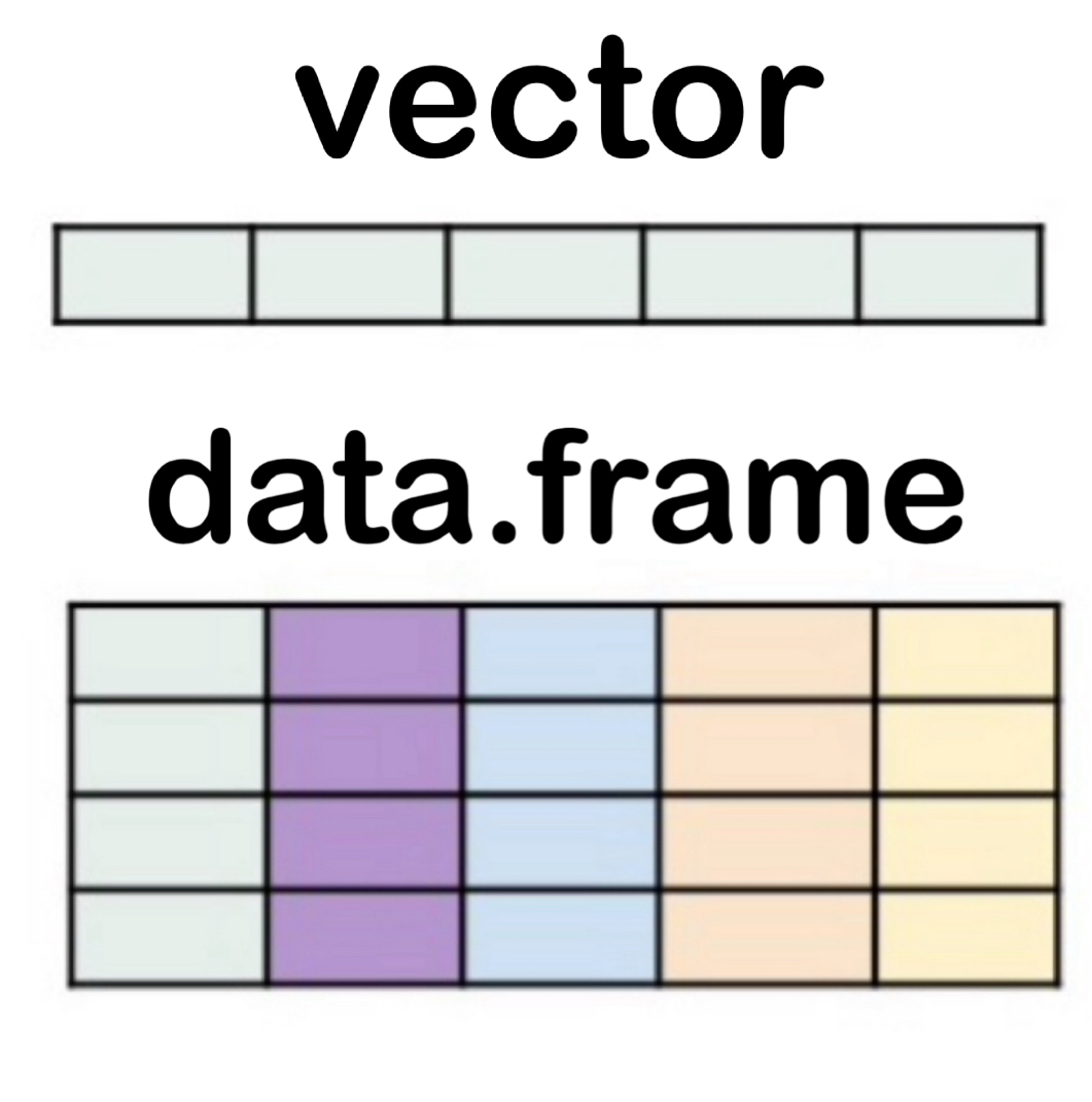
vector → a single column of values, all of the same type
- Example:
  - c(1, 2, 3)
  - c("red", "blue", "green")
data.frame → a table with rows and columns, where each column can be a different type
- Example: one column with names, another with ages
- A data.frame is basically several vectors put together side by side.

Data Types

orig_number <- 4.39898498
class(orig_number)

mod_number <- as.integer(orig_number)
class(mod_number)

# Logical values (TRUE/FALSE) 
  # can convert to numbers:
  # TRUE converts to 1; 
  # FALSE does to 0.
as.numeric(TRUE)
as.numeric(FALSE)

Values have different data types (e.g., numeric, integer, character, factor, logical).
Sometimes we need to convert (cast) a value from one type to another.
Use built-in functions like:
- as.character() → convert to character
- as.integer() → convert to whole numbers
- as.numeric() → convert to numbers with decimals
- as.factor() → convert to categorical (factor)

Data Types - Character

myname <- "my_name"
class(myname) # returns the data **type** of an object.

Strings (text) are stored as the data type character.
Wrap text in either double quotes (" ") or single quotes (' ').
Example: "hello" or 'hello'
Most IDEs, including Posit Cloud (RStudio), will auto-complete the closing quote when you type the first one.

Data Types - Numbers

favorite.integer <- as.integer(2)
class(favorite.integer)

favorite.numeric <- as.numeric(8.8)
class(favorite.numeric)

Numbers can belong to different classes.
The two most common are:
- integer → whole numbers (e.g., 2, -5, 100)
- numeric → numbers with decimals (e.g., 8.8, -3.14, 0.5)

Data Types - Logical (`TRUE`/`FALSE`)

class(TRUE)
class(FALSE)

favorite.numeric == 8.8
favorite.numeric == 9.9
class(favorite.numeric == 8.8)

Logical values represent TRUE or FALSE.
The operator == is used to test for equality.
Example:
- favorite.numeric == 8.8 returns TRUE
- favorite.numeric == 9.9 returns FALSE

Data Types - Vectors

a <- 1:10   # create a sequence using the colon operator
b <- c("3", 4, 5)   # mixing numbers and text
beers <- c("BUD LIGHT", "BUSCH LIGHT", "COORS LIGHT", 
           "MILLER LITE", "NATURAL LIGHT")
length(beers)
class(a)
class(b)
class(beers)

A vector is a one-dimensional data structure in R.
All elements in a vector must be of the same type (numeric, character, or logical).
If types are mixed, R will coerce them to a common type (e.g., numbers become text in b).
The function c(...) (combine or concatenate) creates a vector by putting values together in order.
The function length() returns the number of elements in an object.

Data Types - Factors

beers <- as.factor(beers)
class(beers)

levels(beers)
nlevels(beers)

Factors are used to store categorical data (data that falls into groups or categories).
Internally, R stores factors as integers with a text label for each unique value (for speed and efficiency).
Example: if you have a factor of "Freshman", "Sophomore", "Junior", and "Senior" student classifications, R stores them as numbers (e.g., 1, 2, 3, 4) but displays the labels.
Functions:
- levels() → shows the categories (unique labels)
- nlevels() → shows how many categories there are

Workflow: Quotation marks, parentheses, and `+`

x <- "hello

Quotation marks and parentheses must always come in pairs.
If one is missing, the R Console will show a continuation prompt: +
- This means R is still waiting for more input and doesn’t think your command is finished.

⚙️ Functions

A function is a reusable piece of code: it takes input (parameters) and produces output (results).
R comes with many built-in functions (e.g., sum(), mean()).
You can also write your own functions in R.
- In our course, we will use only built-in functions. m

Functions, Arguments, and Parameters

library(tidyverse)

# The function `str_c()`, provided by `tidyverse`, concatenates characters.
str_c("Data", "Analytics")
str_c("Data", "Analytics", sep = "!")

A function is used by writing its name followed by parentheses ().
A function can take inputs, called arguments, much like a recipe takes ingredients.
Arguments are placed inside the parentheses, separated by commas.
A parameter is the name that represents an expected argument in the function definition.
A default argument is a value that R automatically uses for a parameter if no value is provided when calling the function.

Workflow: Accessing Package Objects/Functions

# Access an object directly from a package
ggplot2::mpg   # PACKAGE_NAME::DATA_FRAME_NAME

# Call a function directly from a package
ggplot2::ggplot()   # PACKAGE_NAME::FUNCTION_NAME

Use the double colon :: operator when you want to access:
- A data frame from a specific package (e.g., ggplot2::mpg)
- A function without loading the entire package (e.g., ggplot2::ggplot())
✅ This can be useful because:
- It avoids name conflicts if two packages have functions with the same name.
- It saves time and memory by letting you call just one function or dataset without loading the entire package.

Math Algebra

( 3 + 4 )^2
3 + 4^2
3 + 2 * 4^2
3 + 2 * 4 + 2
(3 + 2) * (4 + 2)

All of the basic operators with parentheses we see in mathematics are available to use.
R follows the standard order of operations (PEMDAS): Parentheses → Exponents → Multiplication/Division → Addition/Subtraction.
This allows R to be used for a wide range of mathematical calculations.

Math functions

5 * abs(-3)
sqrt(17) / 2
exp(3)
log(3)
log(exp(3))
exp(log(3))

R has many built-in mathematical functions that facilitate calculations and data analysis.

abs(x): the absolute value $|x|$
sqrt(x): the square root $\sqrt{x}$
exp(x): the exponential value $e^x$, where $e = 2.718...$
log(x): the natural logarithm $\log_{e}(x)$, or simply $\log(x)$

Vectorized Operations

a <- c(1, 2, 3, 4, 5)
b <- c(5, 4, 3, 2, 1)

a + 5
a - 5
a * 5
a / 5

a + b
a - b
a * b
a / b

sqrt(a)

Vectorized operations apply a function to every element of a vector automatically, without the need to write a loop.
- Most functions in R are vectorized, meaning they operate element-wise on entire vectors.
- This makes R code more efficient, concise, and well-suited for data analysis and manipulation.

Classwork: R Basics

Try it out → Classwork 4: R Basics I

Descriptive Statistics

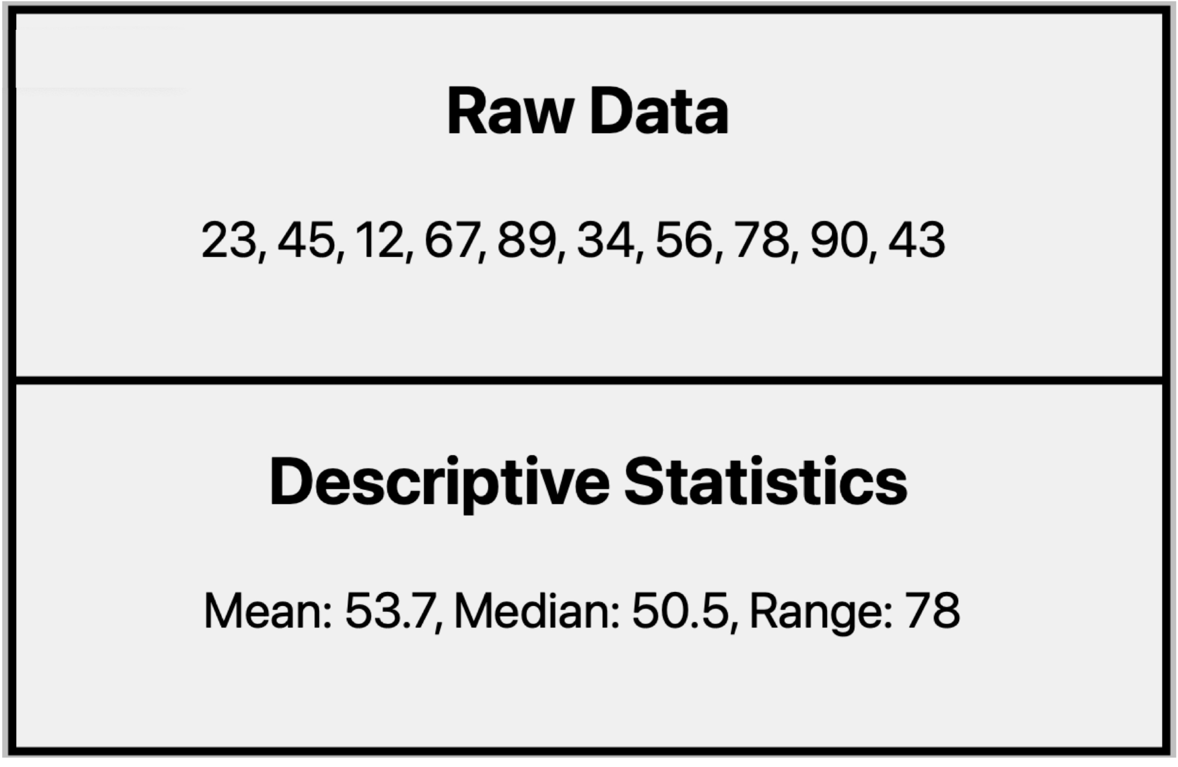
What can descriptive statistics tell us about this dataset?

They condense data into clear, manageable summaries, making it easier to understand the key characteristics of a dataset.
They reveal important patterns, trends, and relationships that may not be immediately obvious from raw numbers.

Descriptive Statistics in Practice

Checking data quality
- Helps spot numbers that don’t seem to fit with the rest of the data.
- Example: If most grocery bills are between $50–$150 but one record shows $10,000, it may be a mistake in recording.
Laying the foundation for analysis
- Gives simple summaries that can be used for deeper study later.
- Example: Knowing both the average and the range of grocery bills helps us understand typical spending patterns.
Supporting data visualization
- Provides clear numbers that make charts and graphs easier to understand.
- Example: Showing the average and range of grocery bills is much simpler than listing every single receipt.

Measures of Central Tendency

Measures of centrality are used to describe the central or typical value in a given vector.
- They represent the “center” or most representative value of a data set.
To describe this centrality, several statistical measures are commonly used:
- Mean: The arithmetic average of all values in the data set.
- Median: The middle value when the data set is ordered from least to greatest.
- Mode: The most frequently occurring value in the data set.

Measures of Central Tendency - Mean

\[ \overline{x} = \frac{x_{1} + x_{2} + \cdots + x_{N}}{N} \]

x <- c(60, 70, 80, 90, 100)
sum(x)
mean(x)

The arithmetic mean (or simply mean or average) is the sum of all the values divided by the number of observations in the data set.
- mean() calculates the mean of the values in a vector.
- For a given vector $x$, if we happen to have $N$ observations $(x_{1}, x_{2}, \cdots , x_{N})$, we can write the arithmetic mean of the data sample as above.

Measures of Central Tendency - Weighted Mean

\[ \begin{align} \overline{x}_{w} &= \frac{w_{1}x_{1} + w_{2}x_{2} + \cdots + w_{N}x_{N}}{w_{1} + w_{2} + \cdots + w_{N}} \end{align} \]

The weighted mean assigns different levels of importance (weights) to each value.
- Each value $x_{i}$ is multiplied by its weight $w_{i}$, and then divided by the sum of the weights.
This is useful when some values contribute more than others (e.g., test scores with different weightings).

Measures of Central Tendency - Median

x <- c(60, 70, 80, 90, 100)
median(x)

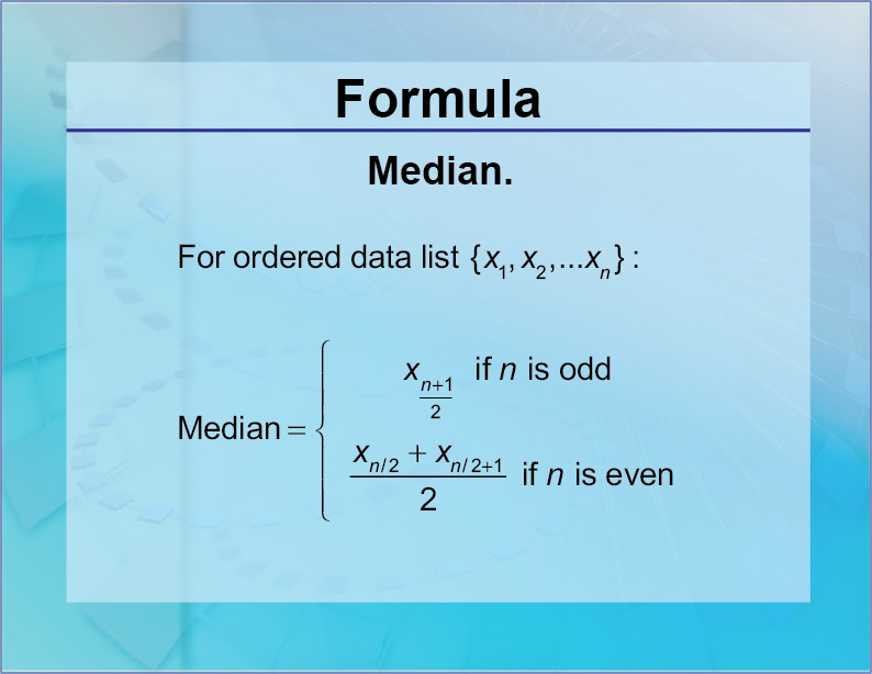
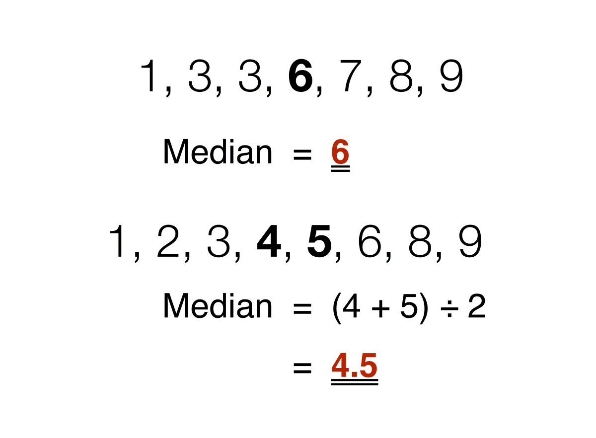
The median is the middle value in a vector—half the numbers are smaller and half are larger.
- median() calculates the median of the values in a vector.
The median is less sensitive to extreme values than the mean.

Measures of Central Tendency - Mode

The mode is the value(s) that occurs most frequently in a given vector.
Mode can be useful, although it is often not a very good representation of centrality.
The R package, modeest, provides the mfw(x) function that calculate the mode of values in vector x.

Measures of Dispersion

Measures of dispersion are used to describe the degree of variation in a given vector.
- They are a representation of the numerical spread of a given data set.
To describe this dispersion, a number of statistical measures are developed
- Range
- Variance
- Standard deviation
- Quartile

Measures of Dispersion - Range

\[ (\text{range of x}) \,=\, (\text{maximum value in x}) \,-\, (\text{minimum value in x}) \]

x <- c(60, 70, 80, 90, 100)
max(x)
min(x)
range <- max(x) - min(x)

The range is the difference between the largest and the smallest values in a given vector.
- max(x) returns the maximum value of the values in a given vector $x$.
- min(x) returns the minimum value of the values in a given vector $x$.

Measures of Dispersion - Variance

\[ \overline{s}^{2} = \frac{(x_{1}-\overline{x})^{2} + (x_{2}-\overline{x})^{2} + \cdots + (x_{N}-\overline{x})^{2}}{N-1}\;\, \]

x <- c(60, 70, 80, 90, 100)  
var(x)

The variance measures how far each data point deviates from the mean, on average (in squared units).
- The larger the variance, the more spread out the data are from the mean.
- Variance squares deviations so that negative and positive differences do not cancel out.
var(x) calculates the variance of the values in a vector x.

Measures of Dispersion - Standard Deviation

\[ \overline{s} = \sqrt{ \left( \frac{(x_{1}-\overline{x})^{2} + (x_{2}-\overline{x})^{2} + \cdots + (x_{N}-\overline{x})^{2}}{N-1}\;\, \right) } \]

x <- c(60, 70, 80, 90, 100)
sd(x)

The standard deviation (SD) is the square root of the variance, expressed in the same unit as the data.
- A low SD suggests values are tightly clustered around the mean, while a high SD suggests greater variability.
- SD is often more useful than variance because it is easier to interpret and directly comparable to the mean.
sd(x) calculates the standard deviation of the values in a vector x.

Measures of Dispersion - Quartiles

quantile(x, 0)    # the minimum
quantile(x, 0.25) # the 1st quartile (Q1)
quantile(x, 0.5)  # the 2nd quartile (Q2, median)
quantile(x, 0.75) # the 3rd quartile (Q3)
quantile(x, 1)    # the maximum

A quartile is a quarter of the number of data points ($N$) in a given vector.
To compute quartiles:

Sort the data in ascending order.
Split into four groups with equal number of data points (or as close as possible if dividing $N$ by 4 leaves a remainder).

Measures of Dispersion – Interquartile Range

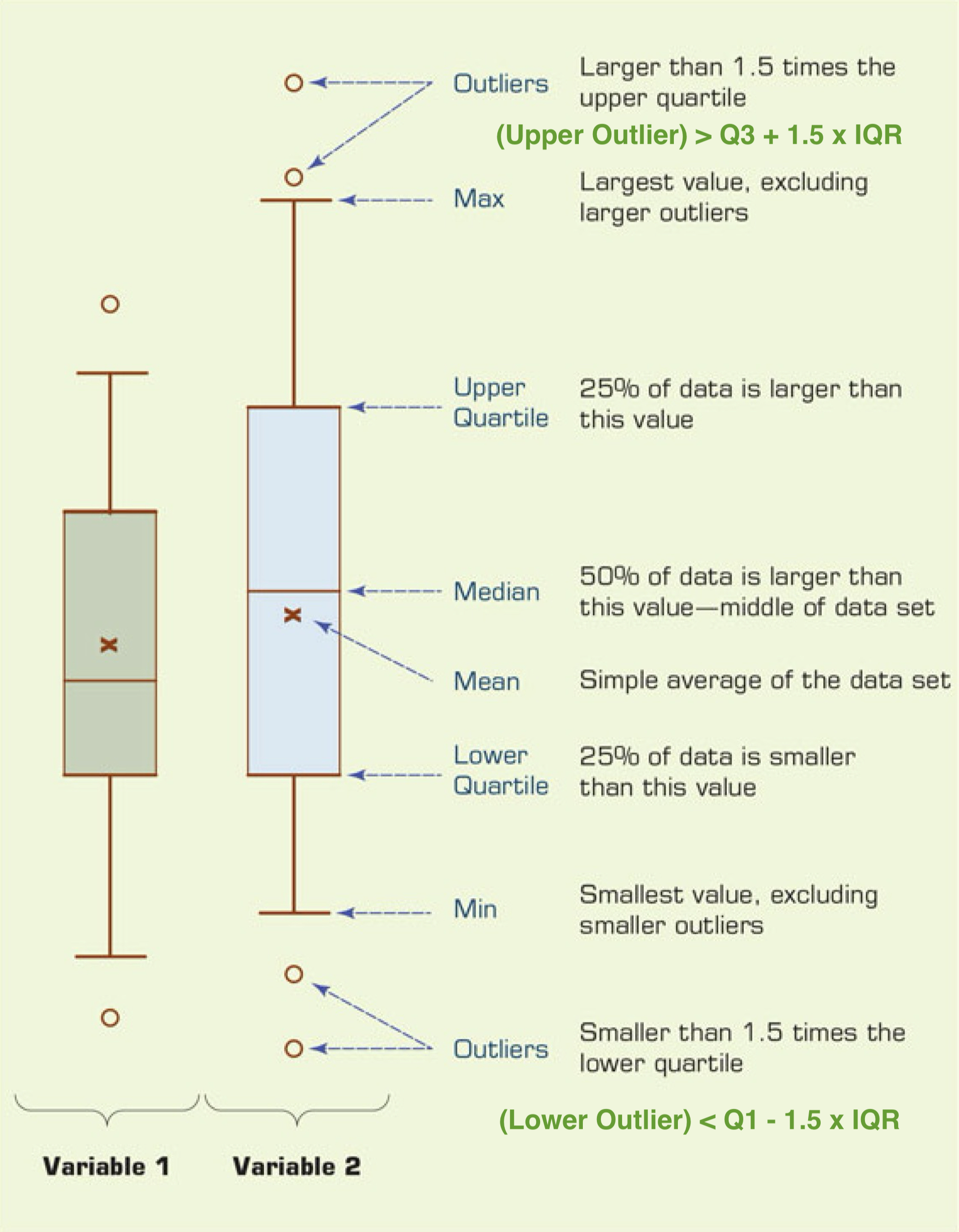
Boxplot

The interquartile range (IQR) is $IQR = Q3 - Q1$.
- It measures the spread of the middle 50% of the data.
- A popular way to visualize quartiles and the IQR is a boxplot.
Why quartiles are useful
- Quartiles show whether the data are more spread out in the lower half or the upper half of the dataset.
- Quartiles are less sensitive to extreme values (outliers) than the mean.

Accessing a Subset of a `vector`

A key part of working with a vector is knowing how to index them.
- Indexing allows you to filter and extract subsets of data for further analysis.
For vectors, there are three common ways to index:

Single index

vec[n]   # element at position n

Multiple indices

vec[c(i, j, k)]   # elements at positions i, j, and k

Logical indexing

vec[condition]   # elements where condition is TRUE

Positional Indexing

An index is a positional reference (e.g., 1, 2, 3) used to access individual elements within data structures like a vector.

my_vector <- c(10, 20, 30, 40, 50, 60)

my_vector[2]
my_vector[4]
my_vector[6]

In R, the index is positive integer, starting at 1.

A Vector of Indices

Selecting multiple elements by providing a vector of indices

my_vector <- c(10, 20, 30, 40, 50, 60)

my_vector[ c(3,4,5) ]
my_vector[ 3:5 ]

Logical Indexing

Using a logical condition to filter elements of a vector.

my_vector <- c(10, 20, 30, 40, 50, 60)

# Filter elements greater than 10
is_greater_than_10 <- my_vector > 10  # Creates logical vector
my_vector[ is_greater_than_10 ]

Classwork: R Basics

Try it out → Classwork 5: R Basics II

Lecture 5

Posit Cloud & R Packages

Posit Cloud

🚀 Getting Started with Posit Cloud

Posit Cloud Environment

Posit Cloud Environment

Posit Cloud Environment

Posit Cloud Environment

📦 R Packages

🌐 tidyverse

📦 Installing R Packages with install.packages("packageName")

📂 Loading R Packages with library(packageName)

Workflow for R packages: Install → Load → Use

Workflow: Naming and File Management

Workflow: Code and comment style

Workflow: Shortcuts in Posit Cloud

Workflow: Shortcuts in Posit Cloud

Workflow: Shortcuts in Posit Cloud

Workflow: Auto-completion

Workflow: STOP icon

Posit Cloud Options Setting

R Programming Basics

Values, Variables, and Data Types

Values, Variables, and Data Types

Assignment

Assignment

Data Types

Data Containers

Data Types

Data Types - Character

Data Types - Numbers

Data Types - Logical (TRUE/FALSE)

Data Types - Vectors

Data Types - Factors

Workflow: Quotation marks, parentheses, and +

⚙️ Functions

Functions, Arguments, and Parameters

Workflow: Accessing Package Objects/Functions

Math Algebra

Math functions

Vectorized Operations

Classwork: R Basics

Descriptive Statistics

Descriptive Statistics

Descriptive Statistics in Practice

Measures of Central Tendency

Measures of Central Tendency - Mean

Measures of Central Tendency - Weighted Mean

Measures of Central Tendency - Median

Measures of Central Tendency - Mode

Measures of Dispersion

Measures of Dispersion - Range

Measures of Dispersion - Variance

Measures of Dispersion - Standard Deviation

Measures of Dispersion - Quartiles

Measures of Dispersion – Interquartile Range

Accessing a Subset of a vector

Accessing a Subset of a vector

Positional Indexing

A Vector of Indices

Logical Indexing

Classwork: R Basics

🌐 `tidyverse`

📦 Installing R Packages with `install.packages("packageName")`

📂 Loading R Packages with `library(packageName)`

Data Types - Logical (`TRUE`/`FALSE`)

Workflow: Quotation marks, parentheses, and `+`

Accessing a Subset of a `vector`

Accessing a Subset of a `vector`