Wildfire Smoke Project

Measuring the U.S. Mortality Cost of Canadian Wildfire Smoke

Byeong-Hak Choe

bchoe@geneseo.edu

SUNY Geneseo

September 28, 2026

June 7, 2023

• Smoke from fires in Quebec turned the sky over New York City orange.
• Air quality in parts of the Northeast reached levels usually seen in the most polluted cities in the world.
• Tens of millions of people breathed smoke from fires hundreds of kilometers away.

How many people in the United States did that smoke kill—and how would we know?

Open with the images students remember from June 2023. The point is that the exposure came from far away, which will later become the key to the research design.

A cross-border externality

• Canada makes fire-management decisions; U.S. residents breathe part of the smoke.
• No market or treaty prices this harm.
• U.S. states can exclude wildfire smoke from Clean Air Act compliance under EPA’s exceptional-events rule.

An externality is a cost imposed on people who are not part of the decision. Here the cost crosses a border.

Connect to the course: environmental economics is about costs that markets do not price. Transboundary pollution is a classic example (China to Korea, Indonesia to Singapore).

The research question

How many deaths in the United States does smoke from Canadian wildfires cause, and what are those deaths worth?

Two numbers:

1. Deaths attributable to Canadian smoke (headline year: 2023)
2. Dollars, using the value of a statistical life (VSL)

This is the framing the research team chose (externality-cost-first). Target journals: economics field journals such as the Review of Economics and Statistics or the Journal of the Association of Environmental and Resource Economists.

What we already know

• A 2025 Nature study estimates about 4,100 acute (short-term) U.S. deaths from the 2023 Canadian smoke.
• It is a health-impact assessment: modeled smoke × a slope (extra deaths per unit of smoke) borrowed from studies of other populations.
• Causal studies of U.S. smoke exist, but they use smoke from U.S. fires.
• No study yet uses the ups and downs of Canadian smoke to estimate U.S. deaths.

Our contribution is the slope itself: extra deaths per unit of Canadian smoke, estimated directly from U.S. counties.

Zhang et al. (2025, Nature 645: 672–678): 4,100 (2,600–5,600) acute U.S. deaths; about 33,000 U.S. deaths from longer-term exposure, which is a different quantity. Their acute slope, about 2% more deaths for each additional 10 µg/m³ of smoke (1.021), matches Chen et al. (2021, Lancet Planetary Health).

[Sources]

• Zhang, Q. et al. (2025), Nature.
• Chen, G. et al. (2021), Lancet Planetary Health.

[/Sources]

Why not just correlate smoke and deaths?

• Smoky days are often hot days, and heat kills.
• The weather patterns that grow fires also steer smoke and bring heat.
• Smoke products measure smoke with error.
• People avoid smoke by staying inside.

Which of these make a simple correlation too large, and which make it too small?

Heat makes a simple correlation too large: hot days are often smoky days, and heat kills on its own. Measurement error and avoidance make it too small. So a simple correlation could be wrong in either direction, which is why we need a research design.

A natural experiment in the sky

• Fires burning 1,000+ km away in Canada are unrelated to local conditions in a U.S. county.
• Whether their smoke reaches that county depends on the day’s winds.
• So: Canadian fire activity located upwind of a county predicts its smoke.

Key idea: find something that changes local smoke but has no other path to local deaths.

Design precedents: shifts in wind direction that move pollution from place to place (Deryugina et al. 2019, AER), and the intensity of Indonesian fires as a driver of Singapore’s pollution (Sheldon and Sankaran 2017, AER Papers and Proceedings). The “no other path” condition is an assumption, so the project tests it before looking at deaths (Gate 1).

Recentering: compare with an average fire season

• Some counties are always more exposed, just by geography.
• For each county and month, compute the exposure it would get from the other 22 fire seasons under the same winds.
• Subtract that expected exposure. What remains is the unusual part of this season’s fires.

Think of it as: “more Canadian fire upwind than an average season would put there, with the same weather.”

Borusyak and Hull (2023, Econometrica) show why an exposure index built from a formula must be compared with its expected value. To measure uncertainty, the project reshuffles whole fire seasons across years, so June and July of the same season are never treated as independent.

The design in one line

Step	Data	What it gives
Fires	NASA FIRMS	Canadian fire radiative power, daily
Transport	ERA5 winds (850–700 hPa)	Which way smoke travels each day
Exposure index	Distance and wind weights + recentering	Unusual upwind Canadian fire, county-month
Smoke	CSU kriged smoke PM2.5	Smoke at ground level, 2006–2025
Deaths	CDC WONDER + SEER	Deaths per 100,000, county-month

Two questions: when unusual upwind fire rises, how much do smoke and deaths rise? The rise in deaths divided by the rise in smoke is the slope.

The analysis answers two linked questions with the same county-month data: (1) how much smoke rises when unusual upwind Canadian fire rises, and (2) how much deaths rise. Dividing (2) by (1) gives deaths per µg/m³ of smoke. Answer (2) is also reported on its own, because it does not depend on how smoke is measured.

From slope to deaths to dollars

\[ \text{Deaths} = \underbrace{\text{slope}}_{\text{from our design}} \times \sum_{\text{counties, months}} \underbrace{\text{Canadian smoke}}_{\text{from a smoke model}} \times \text{population} \]

• The slope comes from the research design.
• The Canadian share of smoke comes from EPA’s EMBER model runs for 2023.
• Dollars = deaths × VSL. EPA’s current guidance uses about $10.7 million (2022 dollars).

Be clear with students about what the design estimates (the slope) and what comes from a model (how much of each county’s smoke was Canadian). The project reports several versions of the Canadian share, plus a version built only from the upwind-fire index, beside the headline.

Data build: fires and winds

• FIRMS: 5.4 million cleaned MODIS fire detections, 2003–2025.
• The MODIS record changes processing version in 2023—right on our headline year.
• ERA5: daily winds over North America, requested from Copernicus.
• The request queue slowed to one job every 7–25 minutes, so the team bundled variables into fewer requests.

Because the headline estimate is for 2023, a measurement break in 2023 could masquerade as a real change. The team carries a collection flag and tests for a break against VIIRS satellites.

Data build: smoke and deaths

• Smoke: CSU kriged PM2.5 (2006–2025), Childs smoke PM2.5 (2006–2023), NOAA HMS plume outlines, EPA monitors.
• Deaths: CDC WONDER suppresses counts of 1–9.
• Keep counties with ≥ 20 deaths per month in 1999–2005: 1,640 counties, about 94% of the population.
• Smaller counties enter as one “rest of state” unit per state.

HMS plumes are often high in the sky in the East. A plume overhead is not smoke at breathing height.

Selecting counties on pre-2006 deaths avoids selecting on the outcome we will study. Poisson math: with an average of 20 deaths a month, the chance of 9 or fewer is about 0.5%.

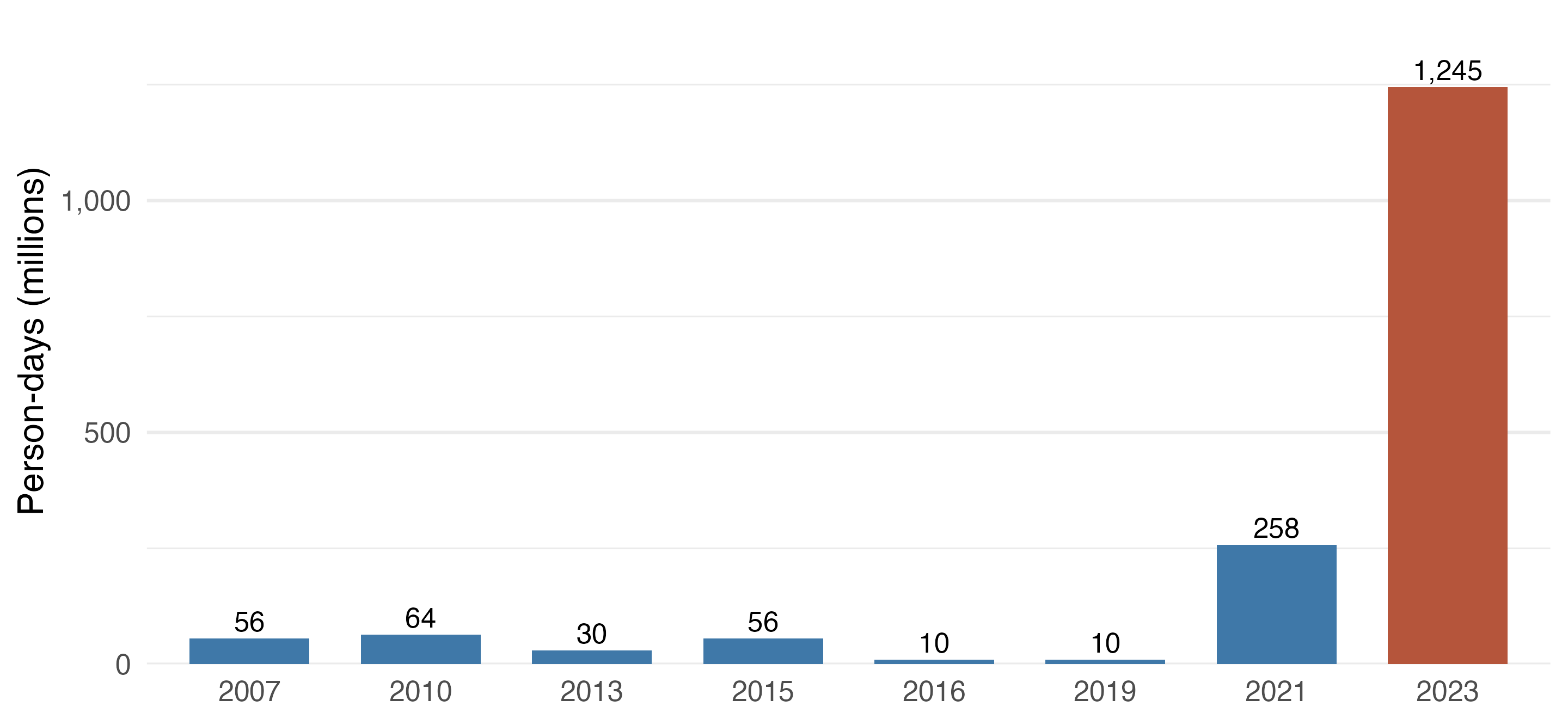
How often does Canadian smoke reach the East?

Person-days of Canadian-dominated smoke above 15 µg/m³ in the eastern U.S., selected years. Preliminary: Childs et al. smoke PM2.5 as a stand-in.

Person-days of Canadian-dominated smoke above 15 µg/m³ in the eastern U.S. (New England, Mid-Atlantic, Great Lakes, Upper Midwest). Preliminary Gate 0 descriptive using Childs et al. smoke PM2.5 as a stand-in; the CSU update adds 2024–2025. 2023 dwarfs every other year, which is why the design uses all twenty seasons rather than 2023 alone. The 2021 episode falls in the excluded COVID window.

Outcome-blind research

• We build and test the design before looking at 2006–2026 deaths.
• Every choice that could change the answer is fixed in advance.
• The plan is registered on Open Science Framework; only then are outcome data merged.

Gate 0 (data) → Gate 1 (index predicts smoke, not heat) → Gate 2 (simulations: can we detect a realistic effect?) → registration → Gate 3 (deaths)

Pre-registration is a commitment device: it prevents the researcher from choosing the specification that gives the most exciting number.

Lessons from the data build

• Data access takes real work: accounts, browser challenges, email-delivered archives, request queues.
• File versions matter: providers re-post files; the pipeline must pick one version on purpose.
• Full disks silently truncate files, so check row counts against the provider.
• Code goes through independent code review until it passes.

Which of these have you already run into in this course?

The build’s code review went 48 → 54 → 70 across three rounds, then a targeted check. Use this to show that reproducible pipelines are built through iteration, not written once.

How you can contribute

• Episode atlas: document each Canadian-smoke episode in the East, 2006–2025.
• Smoke-product comparison: where do HMS, CSU, Childs, and monitors agree?
• EMBER exploration: Canadian share of smoke in June 2023.

• Alerts and attention: NWS air-quality alerts and search interest vs. measured smoke.
• Mechanism literature: adaptation, smoke chemistry, or air conditioning.
• Policy chronology: exceptional-event filings and U.S.–Canada disputes.

All student projects stay outcome-blind: no 2006–2026 mortality data. See the research guide for the full menu and the evidence memo template.

Skills you will practice

• R: tidyverse for panels, sf and terra for spatial data, ncdf4 for NetCDF files
• Spatial joins, population weighting, and time zones (local solar day vs. UTC)
• Reproducible pipelines: scripted downloads, checksums, logs
• Git/GitHub and Quarto for documentation

These are the same skills as the course’s classwork, applied to research-scale data.

Your first two weeks

1. Read the research guide and pick one contribution path.
2. Reproduce one county-day series from raw files and compare it with the project panel.
3. Choose one episode and write a one-page evidence memo.

Bring your memo to our next meeting. We will decide together which question you own for the semester.

Point students to the research guide page on the course site: wildfire-smoke-research-guide.html.

Main takeaways

• Canadian wildfire smoke is an unpriced cross-border externality.
• A simple smoke–death correlation can mislead; distant fires carried by winds give a natural experiment.
• The design estimates the slope; a smoke model and the VSL turn it into deaths and dollars.
• Most of the work is careful data engineering, done before looking at deaths.

What would convince you that our number is more credible than one built on a borrowed slope?

Use the closing question as a short written reflection.