Lecture 6

Map visualization with geom_sf(): wildfire smoke

Byeong-Hak Choe

SUNY Geneseo

September 30, 2026

🗺️ Draw maps

📁 Files for this lecture

Use read_sf() for GeoJSON. Keep county codes, site IDs, and acquisition times as text when reading the CSVs.

# Boundaries and shapes (GeoJSON)
counties <- read_sf("https://bcdanl.github.io/data/wildfire_us_counties_2020.geojson")
states <- read_sf("https://bcdanl.github.io/data/wildfire_us_states_2020.geojson")
provinces <- read_sf("https://bcdanl.github.io/data/wildfire_canada_provinces_2021.geojson")
plumes <- read_sf("https://bcdanl.github.io/data/wildfire_hms_smoke_2023_06.geojson")
nbac <- read_sf("https://bcdanl.github.io/data/wildfire_nbac_burned_area_2023.geojson")

# Data tables (CSV)
smoke_day <- read_csv(
  "https://bcdanl.github.io/data/wildfire_smoke_county_day_2023_06.csv",
  col_types = cols(GEOID = col_character())
)
smoke_month <- read_csv(
  "https://bcdanl.github.io/data/wildfire_smoke_county_month_2006_2025.csv",
  col_types = cols(GEOID = col_character())
)
ember <- read_csv(
  "https://bcdanl.github.io/data/wildfire_ember_county_day_2023_06.csv",
  col_types = cols(GEOID = col_character())
)
aqs <- read_csv(
  "https://bcdanl.github.io/data/wildfire_aqs_pm25_2023_06.csv",
  col_types = cols(GEOID = col_character(), site_id = col_character())
)
fires <- read_csv(
  "https://bcdanl.github.io/data/wildfire_firms_canada_2023.csv",
  col_types = cols(acq_time = col_character())
)
🗺️ Maps with geospatial data

  • A map shows where smoke, fires, and people are located.
  • A familiar boundary can make a regional pattern easy to recognize.
  • A chart often makes rankings and time trends easier to compare.

📋 State smoke averages from county data

state_smoke_june7 <- smoke_day |>
  filter(date == as.Date("2023-06-07")) |>
  left_join(
    counties |>
      st_drop_geometry() |>
      select(GEOID, STUSPS, state_name, region, pop_2020),
    by = "GEOID"
  ) |>
  summarize(
    smoke_pm25 = weighted.mean(smoke_pm25, pop_2020),
    people = sum(pop_2020),
    .by = c(STUSPS, state_name, region)
  )
  • Each state value weights its county estimates by population.

📋 Select states and a national reference

top_state_smoke <- state_smoke_june7 |>
  filter(STUSPS != "DC") |>
  group_by(region) |>
  slice_max(smoke_pm25, n = 5) |>
  ungroup()
national_smoke <- weighted.mean(
  state_smoke_june7$smoke_pm25,
  state_smoke_june7$people
)
  • The chart uses the five states with the highest averages in each Census region.
  • The reference line uses the population-weighted national average.

🔵 Dot plot: set up the axes

p_state0 <- ggplot(
  top_state_smoke,
  aes(
    x = smoke_pm25,
    y = fct_reorder(state_name, smoke_pm25),
    color = region
  )
)
  • fct_reorder() sorts states by their smoke average.
  • The axes compare values without asking readers to compare areas on a map.

➕ Dot plot: add points and a reference line

p_state1 <- p_state0 +
  geom_vline(xintercept = national_smoke,
             color = "grey45",
             linewidth = 0.5) +
  geom_point(size = 2.4) +
  scale_color_brewer(palette = "Dark2") +
  theme_minimal(base_size = 13) +
  labs(x = "Smoke PM2.5 (µg/m³)", y = NULL,
       color = "Census region")

p_state1

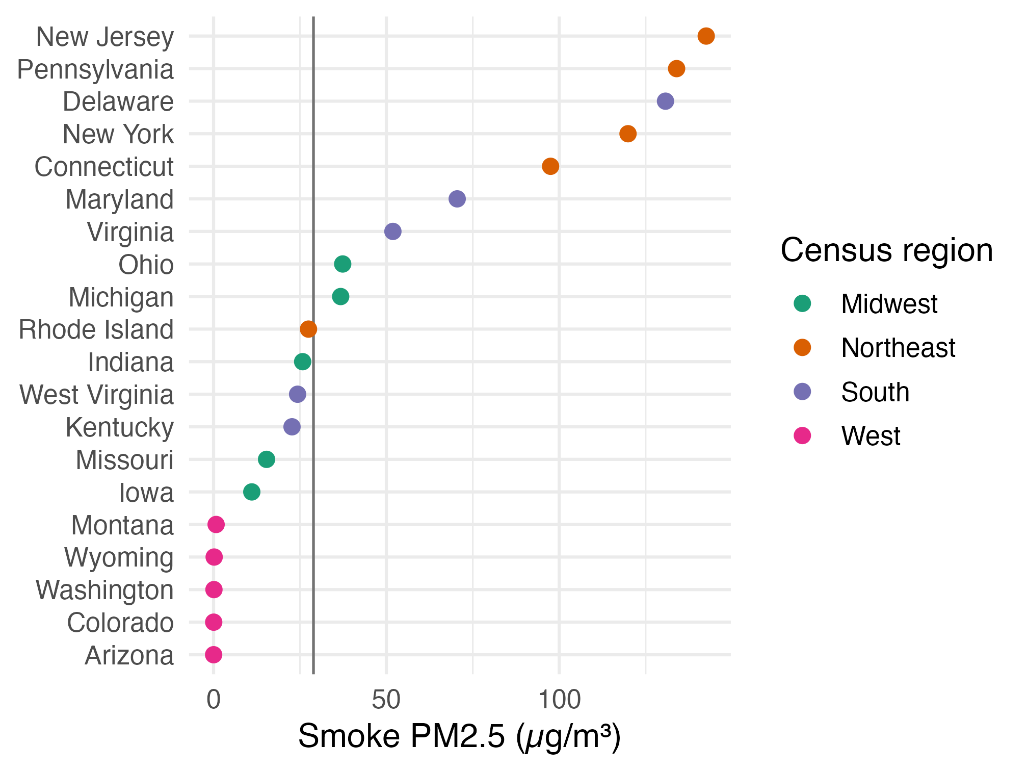
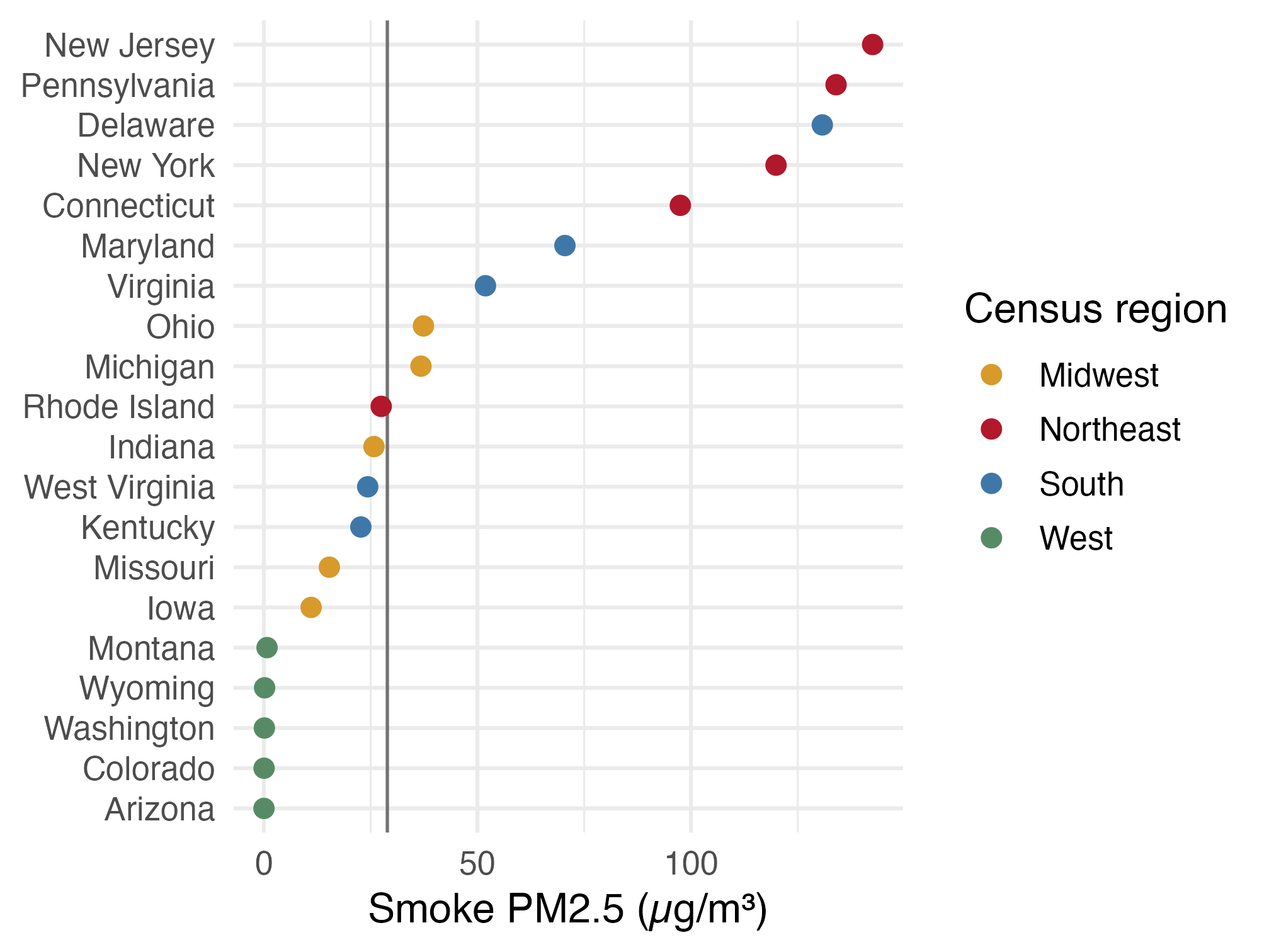
Dot plot of the five highest-smoke states in each Census region on June 7, using a qualitative ColorBrewer palette. New Jersey and Pennsylvania are highest; a vertical line shows the population-weighted national average.

  • The line marks the population-weighted national average: 28.9 µg/m³.
  • Dark2 gives the four regions distinct colors before we fine-tune them.

🎨 Dot plot: apply regional colors

region_colors <- c(
  Midwest = "#d79a2b", Northeast = "#b2182b",
  South = "#3f78a8", West = "#578b67"
)

p_state2 <- p_state1 +
  scale_color_manual(values = region_colors)
p_state2

The same state smoke dot plot with fixed colors for the four Census regions and a vertical national-average reference line.

  • A named color vector replaces the preset palette and keeps each region tied to the same color.

🗂️ Dot plot: facet by Census region

p_state2 +
  facet_wrap(~ region, ncol = 2,
             scales = "free_y") +
  guides(color = "none")

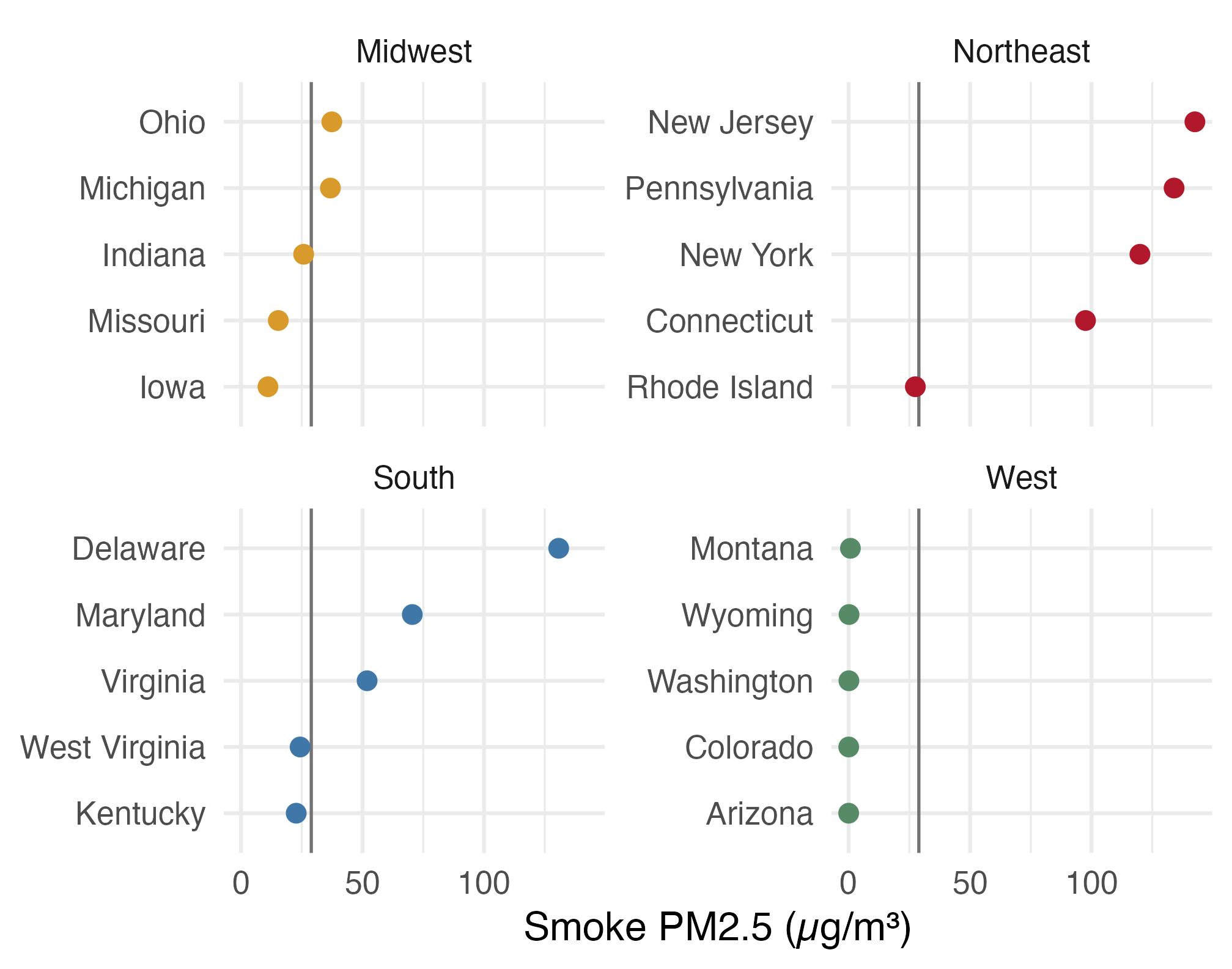
Four small dot plots show the top five June 7 smoke averages within each Census region; the Northeast is far higher than the other regions.

  • The shared x-axis keeps the regional values comparable.
  • A map will show whether the high-smoke states form a geographic cluster.

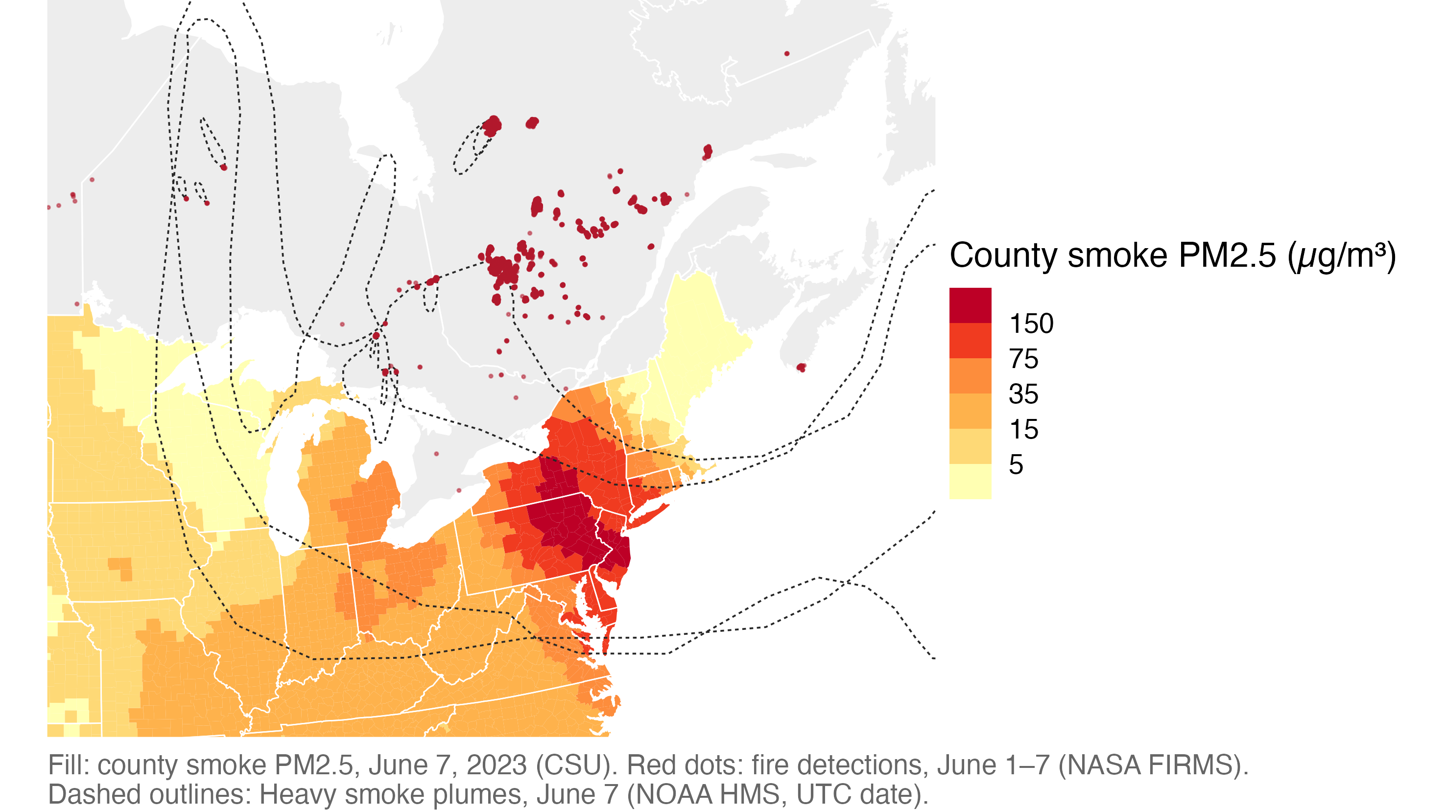
🛰️ June 7, 2023, seen from above

June 7 county smoke is highest around Pennsylvania and New Jersey; fire detections cluster in Quebec, with Heavy plume outlines spanning eastern North America.

Where did this smoke come from? What would you check before trusting this map?

🗺️ A map is geometry plus a projection

  • Points: a fire detection, an air-quality monitor, a city
  • Lines: a road, a river, a flight path
  • Polygons: a county, a smoke plume, a burned area
  • A projection flattens the round Earth onto a flat page, and every projection distorts something

Healy: a map is just shapes drawn in the right order on an x–y plane, plus a projection. The rest is ordinary ggplot.

📋 Plan for today

  • Simple features and projections: read, draw, and flatten boundaries
  • Choropleths and small multiples: join smoke data to county shapes and compare dates
  • Hexagons, points, plumes, and spatial joins
  • When a map is not the best chart

📐 Draw maps with sf

📂 The course files

All files are at https://bcdanl.github.io/data/.

File One row is
wildfire_us_counties_2020.geojson a lower-48 county (3,108, incl. DC)
wildfire_us_states_2020.geojson a state or DC (49)
wildfire_canada_provinces_2021.geojson a province or territory (13)
wildfire_smoke_county_day_2023_06.csv county × day, June 2023
wildfire_smoke_county_month_2006_2025.csv county × month, 2006–2025
wildfire_aqs_pm25_2023_06.csv air monitor × day, June 2023
wildfire_ember_county_day_2023_06.csv county × day, modeled fire PM2.5
wildfire_hms_smoke_2023_06.geojson smoke plume drawn by an analyst, June 2023
wildfire_firms_canada_2023.csv satellite fire detection in Canada, 2023
wildfire_nbac_burned_area_2023.geojson 2023 Canadian fire, outer outline

📁 Read boundaries with read_sf()

library(tidyverse)
library(sf)
library(scales)
library(ggrepel)

course_url <- "https://bcdanl.github.io/data/"

counties  <- read_sf(paste0(course_url, "wildfire_us_counties_2020.geojson"))
states    <- read_sf(paste0(course_url, "wildfire_us_states_2020.geojson"))
provinces <- read_sf(paste0(course_url, "wildfire_canada_provinces_2021.geojson"))
  • read_sf() reads GeoJSON, shapefiles (.shp), and GeoPackages into a tibble.
  • Census and Statistics Canada publish boundary files like these for free.

🔍 An sf object is a tibble with a geometry column

counties |>
  select(GEOID, county_name, pop_2020) |>
  print(n = 3)
Simple feature collection with 3108 features and 3 fields
Geometry type: MULTIPOLYGON
Dimension:     XY
Bounding box:  xmin: -124.7627 ymin: 24.5213 xmax: -66.9499 ymax: 49.3844
Geodetic CRS:  WGS 84
# A tibble: 3,108 × 4
  GEOID county_name    pop_2020                     geometry
  <chr> <chr>             <dbl>           <MULTIPOLYGON [°]>
1 01001 Autauga County    58805 (((-86.9176 32.6642, -86.71…
2 01003 Baldwin County   231767 (((-87.9729 31.1627, -87.94…
3 01005 Barbour County    25223 (((-85.4164 31.6195, -85.74…
# ℹ 3,105 more rows
  • sf = simple features: shapes stored as rows of a table.
  • geometry is a list column: one shape per county.
  • Geometry is sticky: select() keeps it.
  • CRS (coordinate reference system): WGS 84 longitude and latitude.

🖊️ Your first geom_sf()

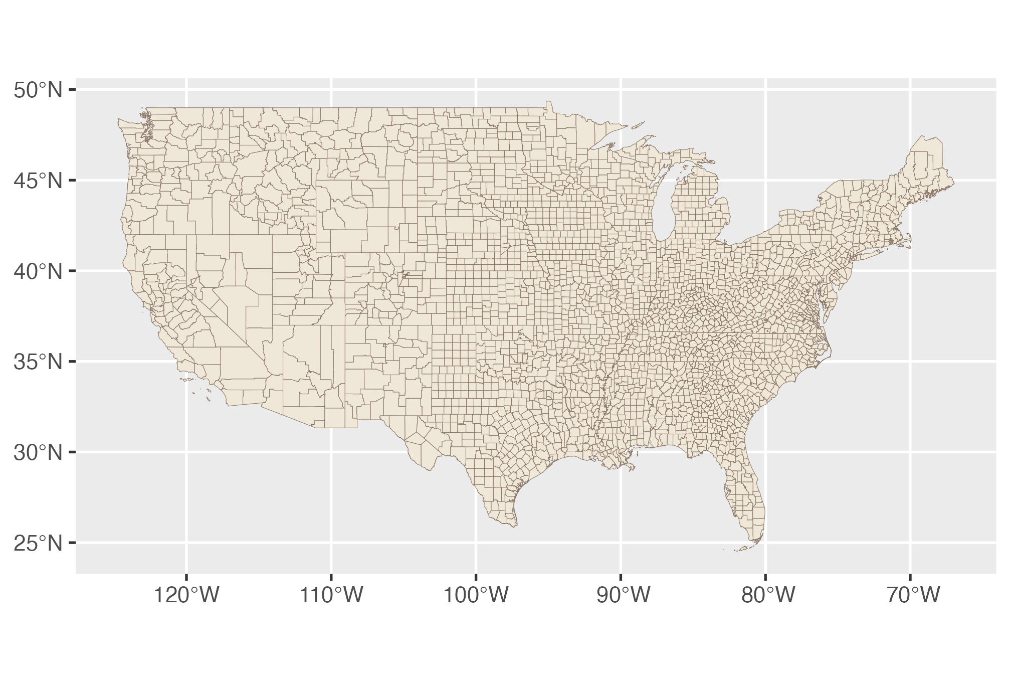
ggplot(counties) +
  geom_sf(fill = "#efe7d8",
          color = "#8b7767",
          linewidth = 0.1)

Map of lower-48 county boundaries, with many small eastern counties and larger western counties.

  • No aes(x, y): geom_sf() finds the geometry column itself.
  • The axes are longitude and latitude in degrees.

🎨 Set a map theme once

theme_set(
  theme_void(base_size = 15) +
    theme(
      legend.position = "bottom",
      legend.title.position = "top",
      legend.key.width = unit(2.4, "lines"),
      plot.title = element_text(face = "bold"),
      strip.text = element_text(size = rel(1)),
      plot.caption = element_text(color = "grey40", hjust = 0),
      plot.caption.position = "plot"
    )
)
  • theme_void() drops axes, grid lines, and the grey panel.
  • theme_set() applies it to every plot after this line.

➕ Style and layer: states over counties

state_lines <- geom_sf(
  data = states, fill = NA,
  color = "grey25", linewidth = 0.25
)

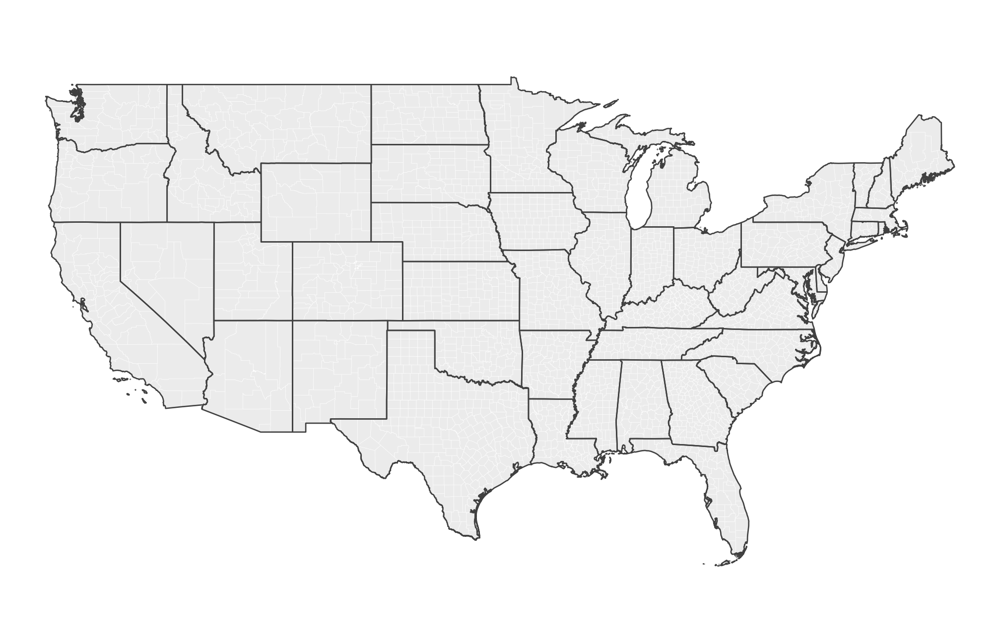
ggplot(counties) +
  geom_sf(fill = "grey92",
          color = "white",
          linewidth = 0.05) +
  state_lines

Lower-48 county outlines in white with darker state borders layered on top.

  • Layers are drawn in order; fill = NA makes states see-through.
  • A saved layer (state_lines) can be added to any later map.

🔗 Dissolve counties into Census regions

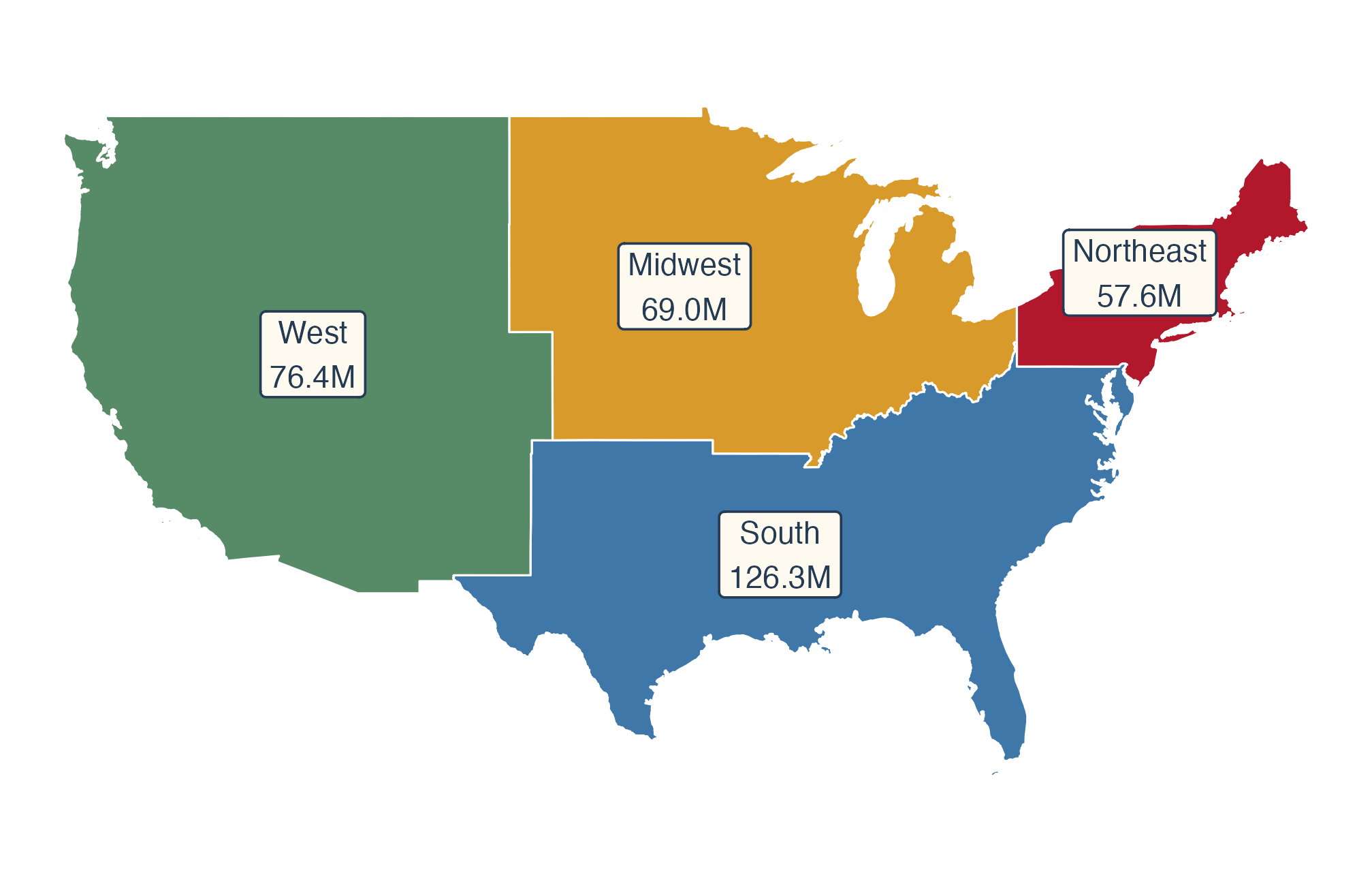
regions <- counties |>
  group_by(region) |>
  summarize(pop = sum(pop_2020))

ggplot(regions) +
  geom_sf(aes(fill = region),
          color = "white", linewidth = 0.3) +
  scale_fill_manual(values = region_colors) +
  geom_sf_label(
    aes(label = paste0(region, "\n",
      number(pop / 1e6, accuracy = 0.1),
      "M")),
    size = 3.2,
    color = "#243b53", fill = "#fffaf0"
  ) +
  guides(fill = "none")

Four colored Census regions labeled West 76.4 million, Midwest 69.0 million, South 126.3 million, and Northeast 57.6 million people.

  • summarize() on an sf object unions the polygons in each group.

🌎 North America: Different Projections

🧭 Which coordinate reference system?

st_crs(counties)$Name
[1] "WGS 84"
st_crs(counties)$epsg
[1] 4326
Code Name Use today
EPSG:4326 WGS 84 longitude/latitude how the files are stored
EPSG:4269 NAD83 longitude/latitude many U.S. federal files
ESRI:102003 USA Contiguous Albers Equal Area lower-48 maps
EPSG:5070 NAD83 / Conus Albers (meters) lower-48 data stored in meters
ESRI:102009 North America Lambert Conformal Conic Canada + U.S. maps

🌐 Longitude–latitude vs. Albers

us_map <- ggplot(states) +
  geom_sf(fill = "grey80", color = "white")

us_map + coord_sf(crs = 4326)

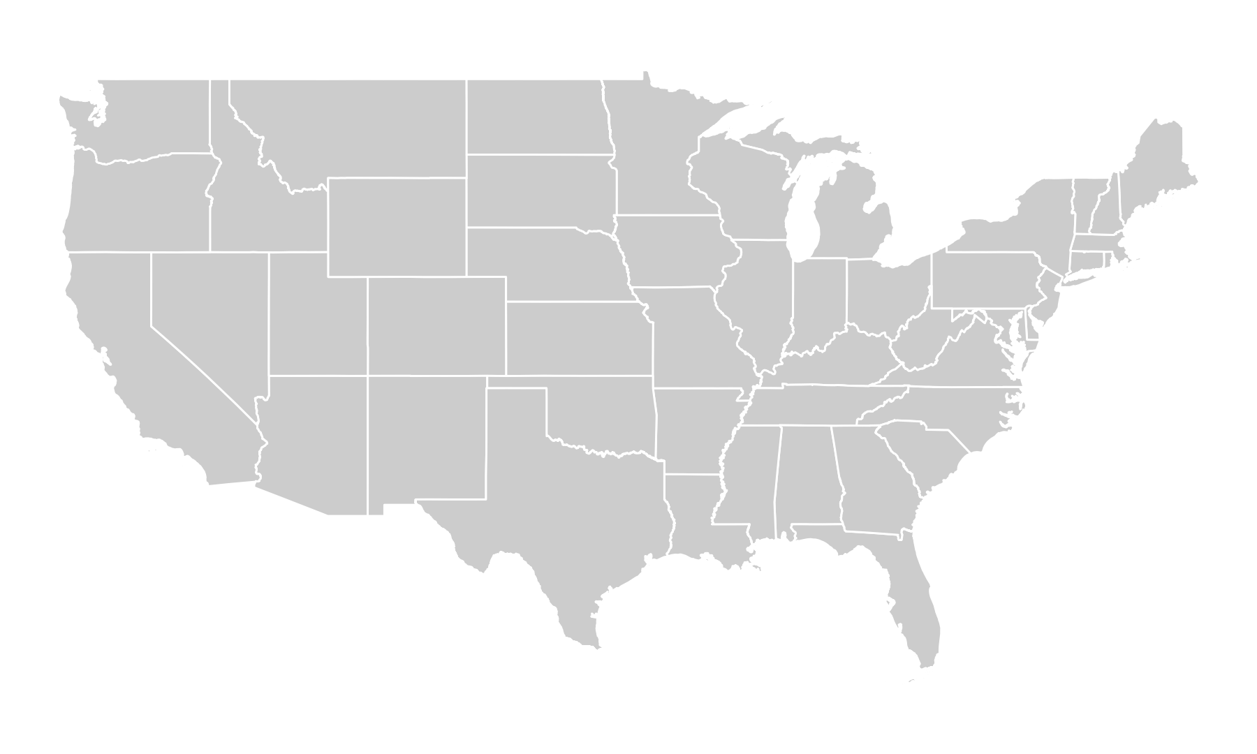
Lower-48 state outlines in longitude and latitude coordinates, giving the country a flatter, wider appearance.

us_map +
  coord_sf(crs = "ESRI:102003")

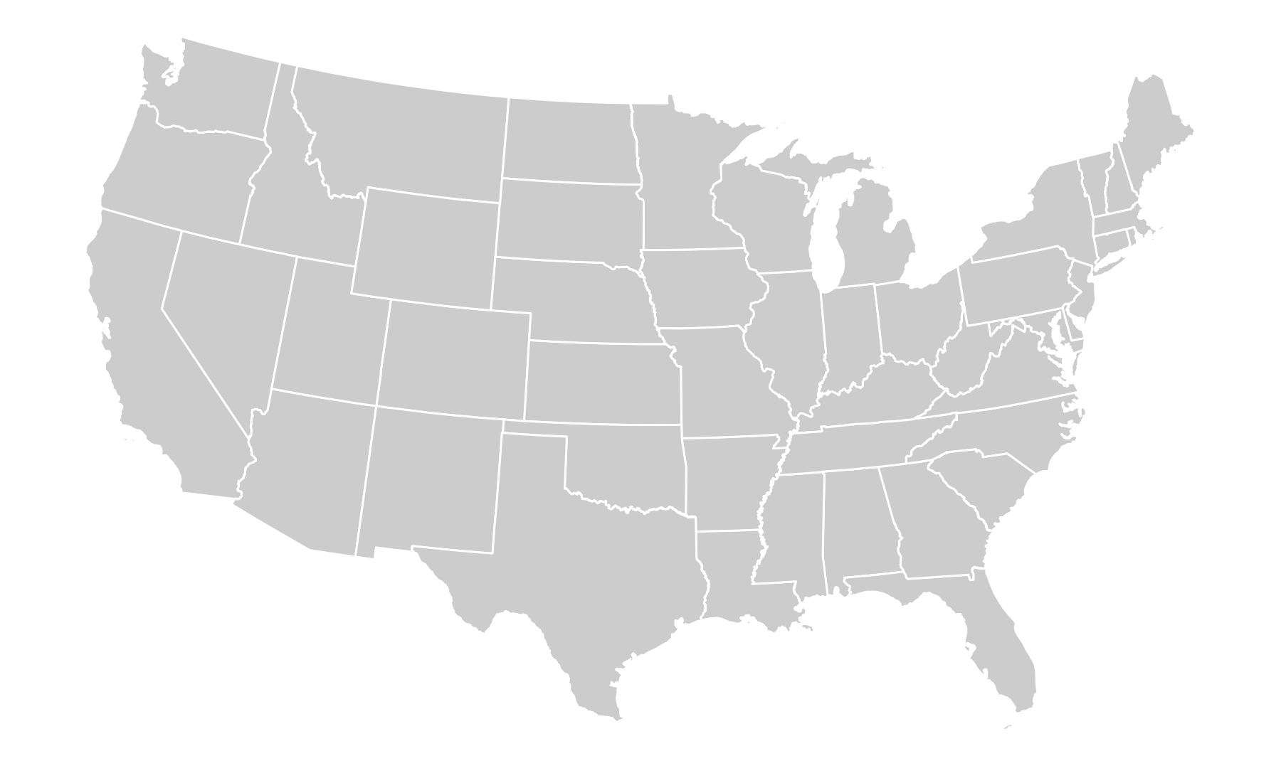
The same lower-48 state outlines in an equal-area Albers projection, with a more curved northern edge.

  • Albers (right) is equal-area: no region gets extra ink.

📐 coord_sf() vs. st_transform()

us_albers <- coord_sf(crs = "ESRI:102003")

counties_5070 <- st_transform(counties, crs = 5070)
st_crs(counties_5070)$Name
[1] "NAD83 / Conus Albers"
st_bbox(counties_5070) |> round()
    xmin     ymin     xmax     ymax 
-2356011   269579  2258155  3172569 
  • coord_sf(): draw in a projection; the data stay in degrees.
  • st_transform(): changes the stored coordinates (here to meters); layers must share a CRS before a spatial join.

🌎 North America in one projection

na_lcc <- coord_sf(crs = "ESRI:102009")

ggplot() +
  geom_sf(data = provinces,
          fill = "#e7d9c4",
          color = "white") +
  geom_sf(data = states,
          fill = "grey80",
          color = "white") +
  na_lcc

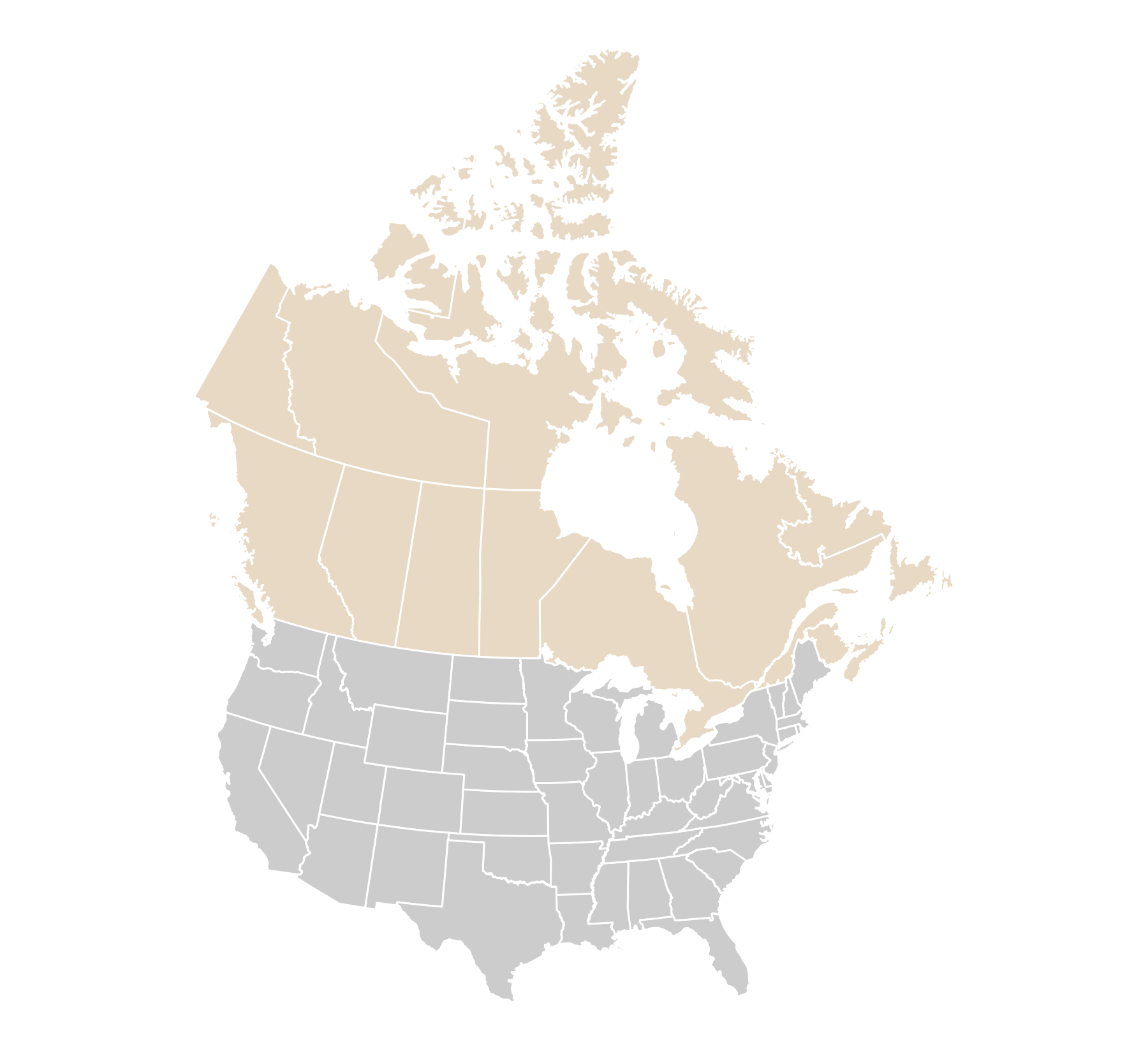
Canadian provinces and U.S. states shown together in a North American projection.

  • One coord_sf() reprojects both layers.

🔎 Zoom with longitude–latitude limits

east_zoom <- coord_sf(
  crs = "ESRI:102009",
  xlim = c(-95, -60), ylim = c(36, 56),
  default_crs = st_crs(4326)
)

ggplot() +
  geom_sf(data = provinces,
          fill = "#e7d9c4", color = "white") +
  geom_sf(data = states,
          fill = "grey80", color = "white") +
  east_zoom

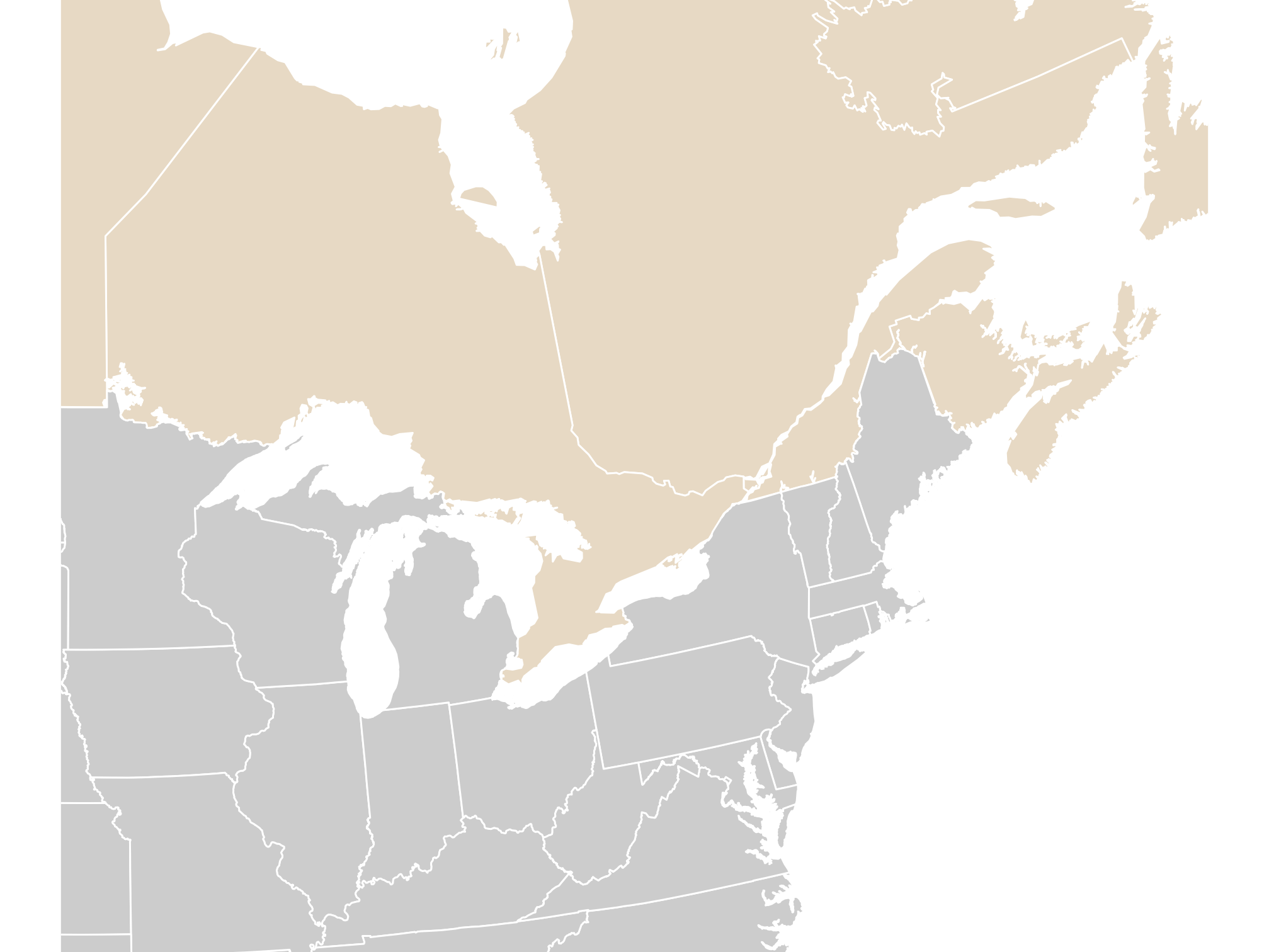
Map zoomed to eastern Canada and the northeastern United States.

  • default_crs = st_crs(4326): “my limits are in degrees.”

🎨 Choropleth Maps

📂 Read the smoke tables with GEOID as text

smoke_day <- read_csv(
  paste0(course_url, "wildfire_smoke_county_day_2023_06.csv"),
  col_types = cols(GEOID = col_character()))
smoke_month <- read_csv(
  paste0(course_url, "wildfire_smoke_county_month_2006_2025.csv"),
  col_types = cols(GEOID = col_character()))
aqs <- read_csv(
  paste0(course_url, "wildfire_aqs_pm25_2023_06.csv"),
  col_types = cols(GEOID = col_character(), site_id = col_character()))
ember <- read_csv(
  paste0(course_url, "wildfire_ember_county_day_2023_06.csv"),
  col_types = cols(GEOID = col_character()))
  • GEOID is a FIPS code: 2-digit state + 3-digit county. "01001" is Autauga County, AL.

PM2.5 = tiny particles (2.5 micrometers or smaller) in the air, measured in micrograms per cubic meter (µg/m³). total_pm25 counts particles from every source; smoke_pm25 is the part above a normal background on days a satellite saw smoke.

⚠️ What a numeric GEOID does to a join

bad_ids <- as.character(as.numeric(smoke_day$GEOID))
head(unique(bad_ids), 3)
[1] "1001" "1003" "1005"
sum(!counties$GEOID %in% bad_ids)
[1] 287
  • 287 counties in six states (AL, AZ, AR, CA, CO, CT) would silently drop out of the join.
  • Join on codes, not names, and keep codes as text (Healy).

🔍 Check the keys before you join

n_distinct(smoke_day$GEOID)
[1] 3108
anti_join(counties, smoke_day, by = "GEOID") |> nrow()
[1] 0
setdiff(smoke_day$GEOID, counties$GEOID)
character(0)
  • Every county has smoke data, and every smoke row has a county.
  • anti_join() returns the rows with no match; we want zero.

Boundaries change. Census data from 2022 on use 9 Connecticut planning regions (09110–09190) in place of the 8 old counties (09001–09015) in our 2020 shapes. Joining newer Connecticut data would leave all 8 counties unmatched, and this anti_join() would show them. Match the boundary year to the data year (Healy).

🔗 Join the table to the geometry

june7 <- smoke_day |>
  filter(date == as.Date("2023-06-07"))

smoke_june7 <- counties |>
  left_join(june7, by = "GEOID")

class(smoke_june7)
[1] "sf"         "tbl_df"     "tbl"        "data.frame"
nrow(smoke_june7)
[1] 3108
  • Put the sf object on the left; the result stays sf, one row per county.

🔵 Fill counties by smoke category

smoke_category <- smoke_june7 |>
  mutate(smoke_band = case_when(
    smoke_pm25 < 15 ~ "<15",
    smoke_pm25 <= 35 ~ "15–35",
    TRUE ~ ">35"
  ) |> factor(levels = c(
    "<15", "15–35", ">35"
  )))

p_band0 <- ggplot(
  smoke_category,
  aes(fill = smoke_band)
) +
  geom_sf(color = NA) + state_lines +
  scale_fill_brewer(
    palette = "YlOrRd",
    name = "Smoke PM2.5 (µg/m³)"
  ) +
  us_albers +
  theme(legend.position = "right")
p_band0

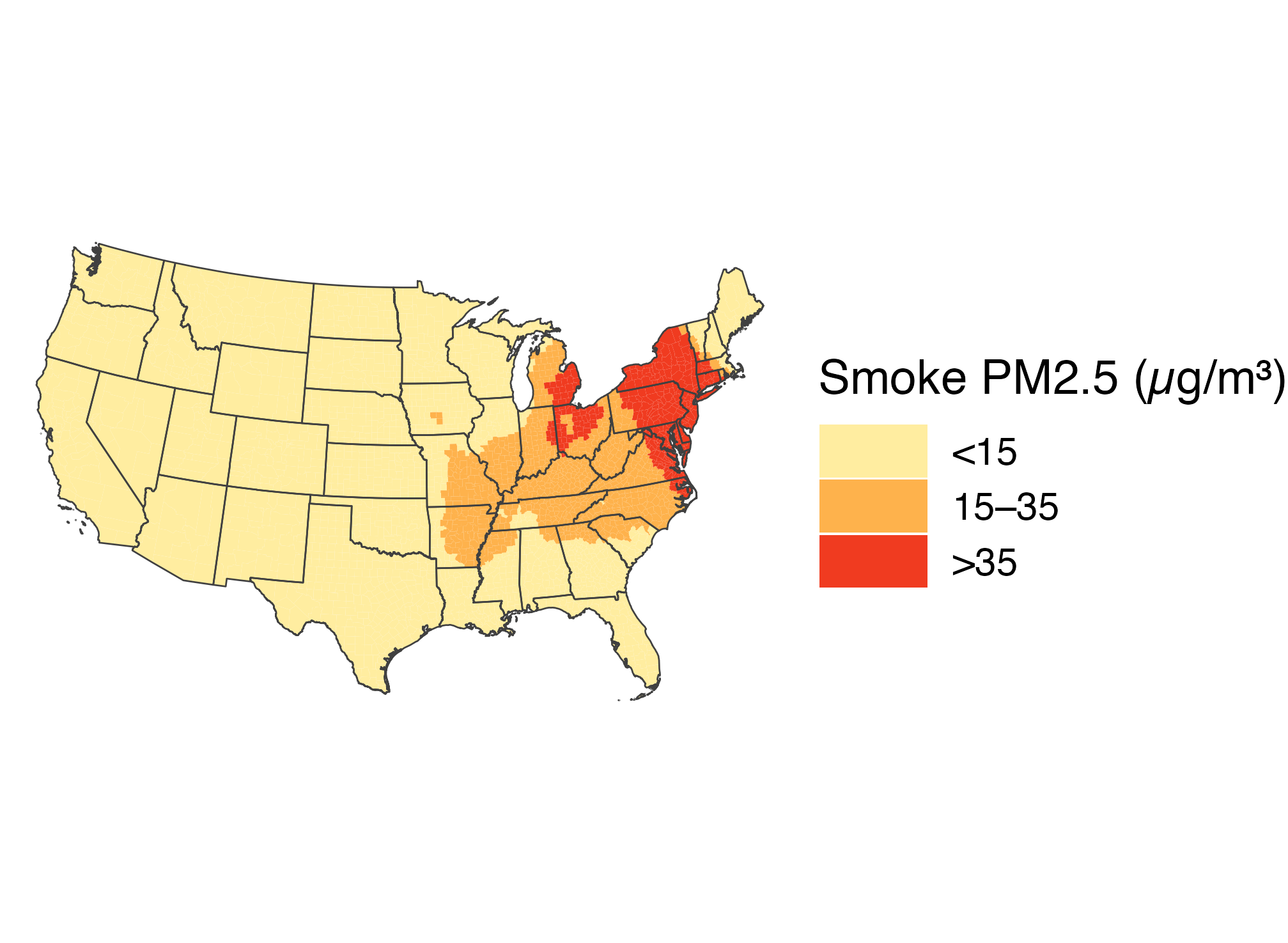
June 7 county smoke grouped into three categories using a yellow-orange-red palette. Dark red high-smoke counties cluster in the Northeast.

  • fill maps an ordered smoke category to color.
  • The category cutoffs are in µg/m³ of the smoke component.
  • YlOrRd orders the colors from pale yellow to dark red.

🎨 Apply colors with scale_fill_manual()

smoke_band_colors <- c(
  "<15" = "#fff7bc",
  "15–35" = "#fdae61",
  ">35" = "#b2182b"
)

p_band1 <- p_band0 +
  scale_fill_manual(
    values = smoke_band_colors,
    name = "Smoke PM2.5 (µg/m³)"
  )
p_band1

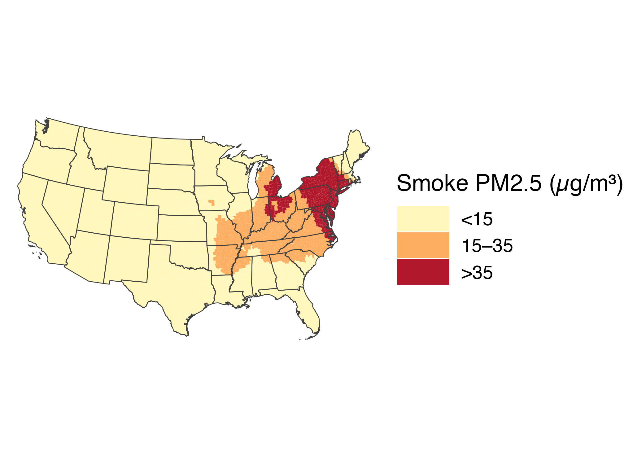
The June 7 three-category smoke map uses pale yellow for under 15, orange for 15 to 35, and dark red for over 35 micrograms per cubic meter.

  • The named vector replaces the preset palette and assigns colors by category label.

🔖 Move the legend below the map

p_band2 <- p_band1 +
  guides(fill = guide_legend(nrow = 1)) +
  theme(legend.position = "bottom")
p_band2

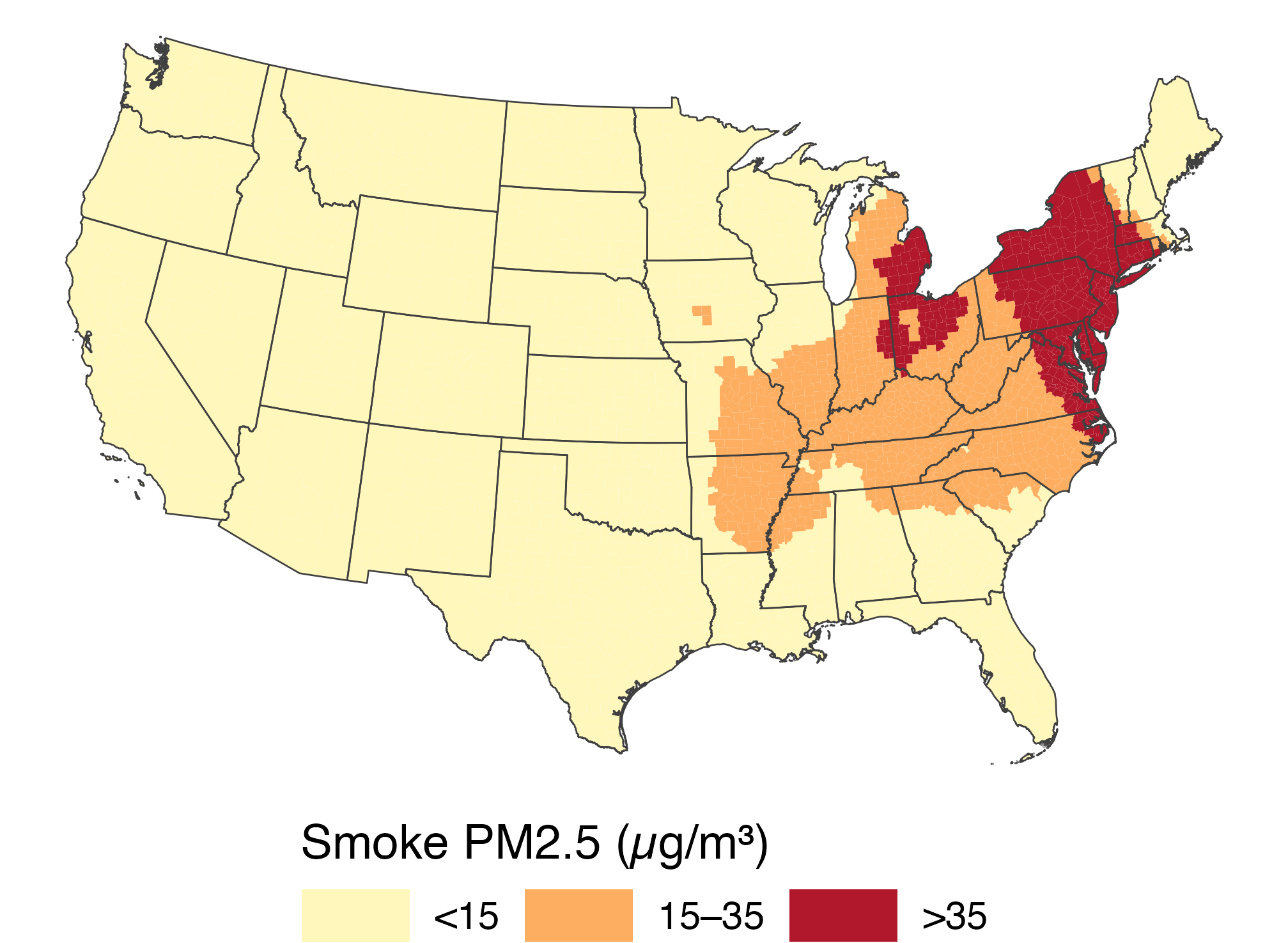
The three-category county smoke map with a single-row legend below the United States.

  • guide_legend(nrow = 1) keeps the three categories in one row.
  • The legend states both the variable and its units.

🔄 Reversing colors changes the message

reversed_colors <- setNames(
  rev(unname(smoke_band_colors)),
  names(smoke_band_colors)
)

p_band0 +
  scale_fill_manual(
    values = reversed_colors,
    name = "Smoke PM2.5 (µg/m³)"
  )

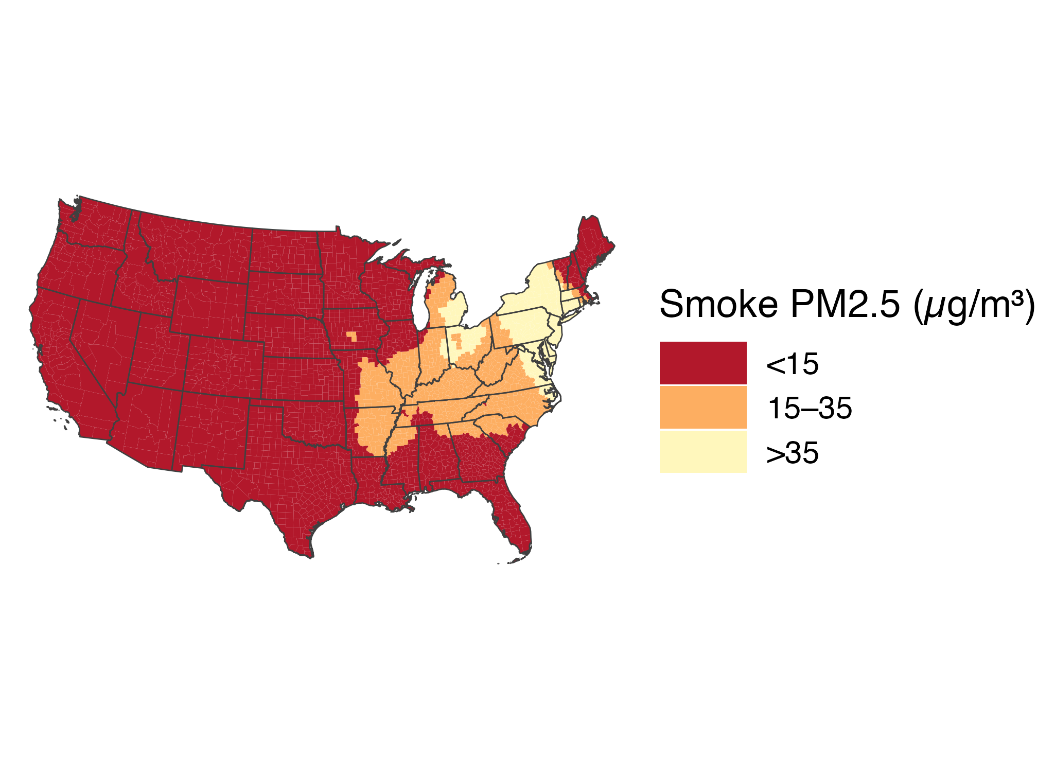
The same June 7 county categories with the palette reversed. Low-smoke counties now look dark and high-smoke counties look pale, showing how color order changes emphasis.

  • The data stayed the same. The dark color now means low smoke.
  • Use a color order that matches what the legend asks readers to notice.

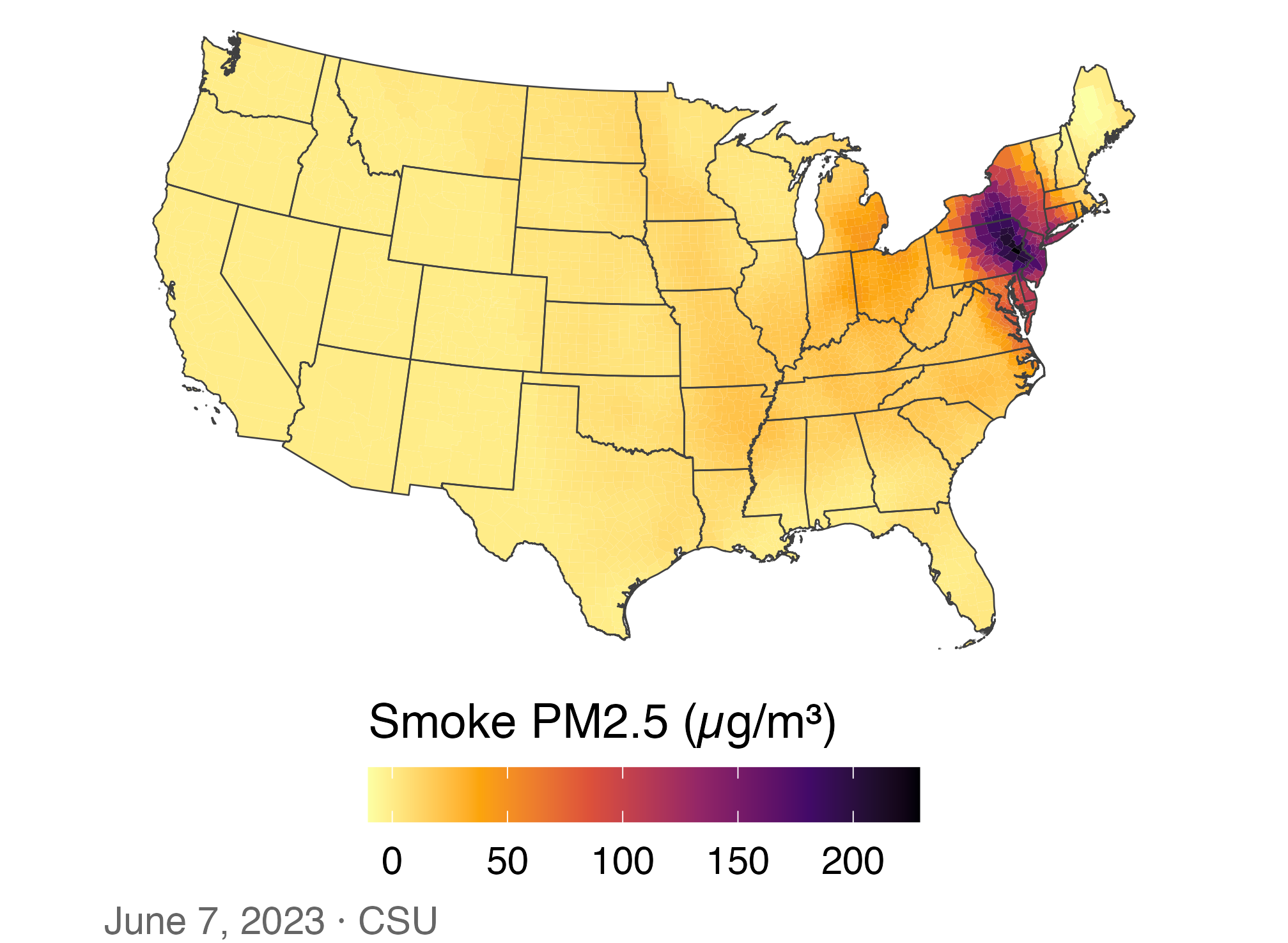
📈 A first choropleth: June 7, 2023

p_smoke0 <- ggplot(smoke_june7,
                   aes(fill = smoke_pm25)) +
  geom_sf(color = NA) + state_lines +
  scale_fill_viridis_c(
    option = "inferno", direction = -1,
    name = "Smoke PM2.5 (µg/m³)"
  ) +
  us_albers +
  labs(caption = "June 7, 2023 · CSU")
p_smoke0

June 7 county smoke PM2.5 on a continuous scale; the darkest counties cluster around Pennsylvania and New Jersey while most of the West is pale.

Most of the country looks the same pale color. Why?

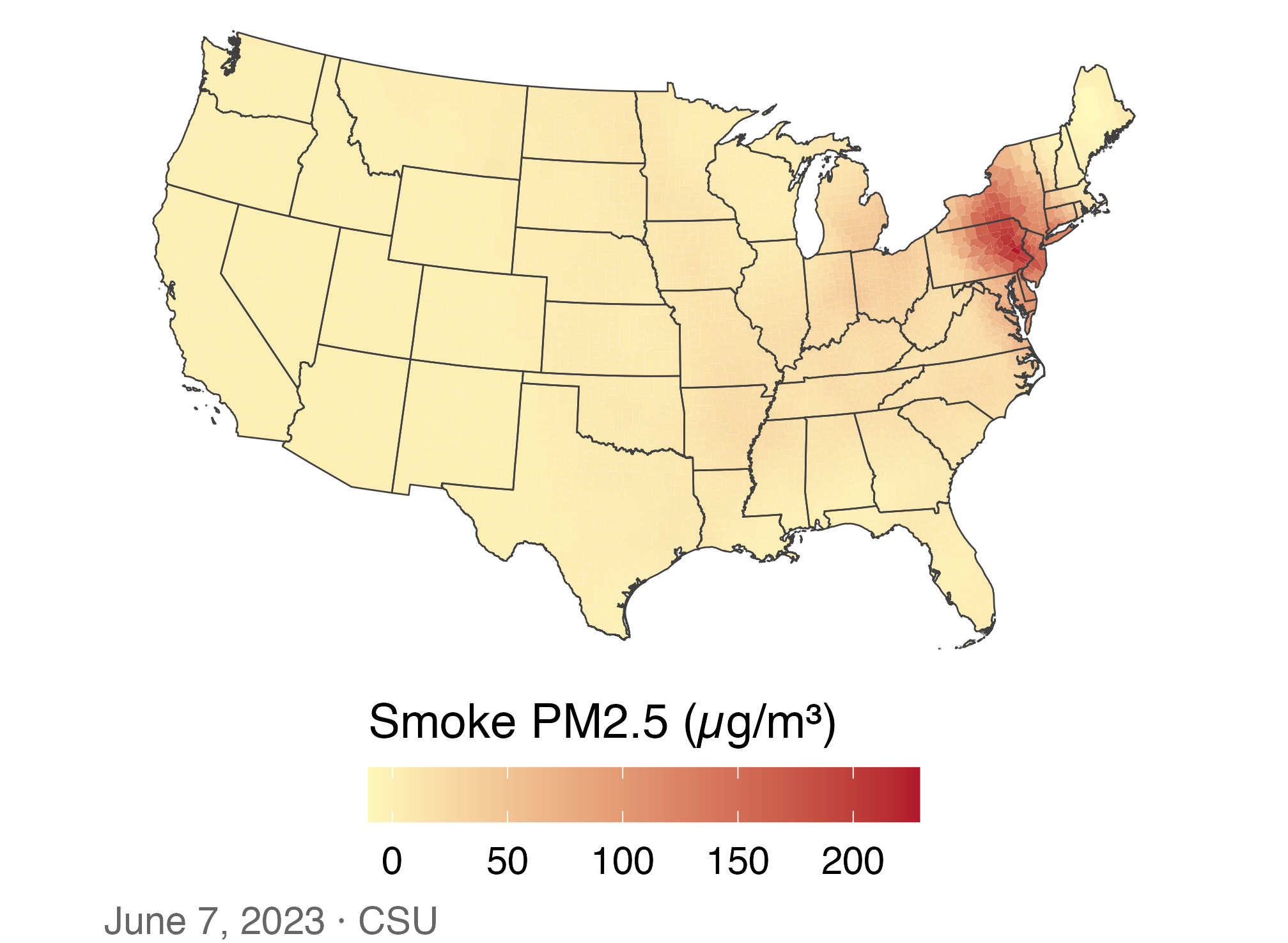
🎨 Set a sequential color gradient

p_smoke0 +
  scale_fill_gradient(
    low = "#fff7bc", high = "#b2182b",
    name = "Smoke PM2.5 (µg/m³)"
  )

June 7 county smoke on a yellow-to-red continuous gradient. Eastern Pennsylvania and nearby counties are darkest, while most counties are pale.

  • scale_fill_gradient() controls the low and high colors.
  • The few extreme counties still compress most of the scale.

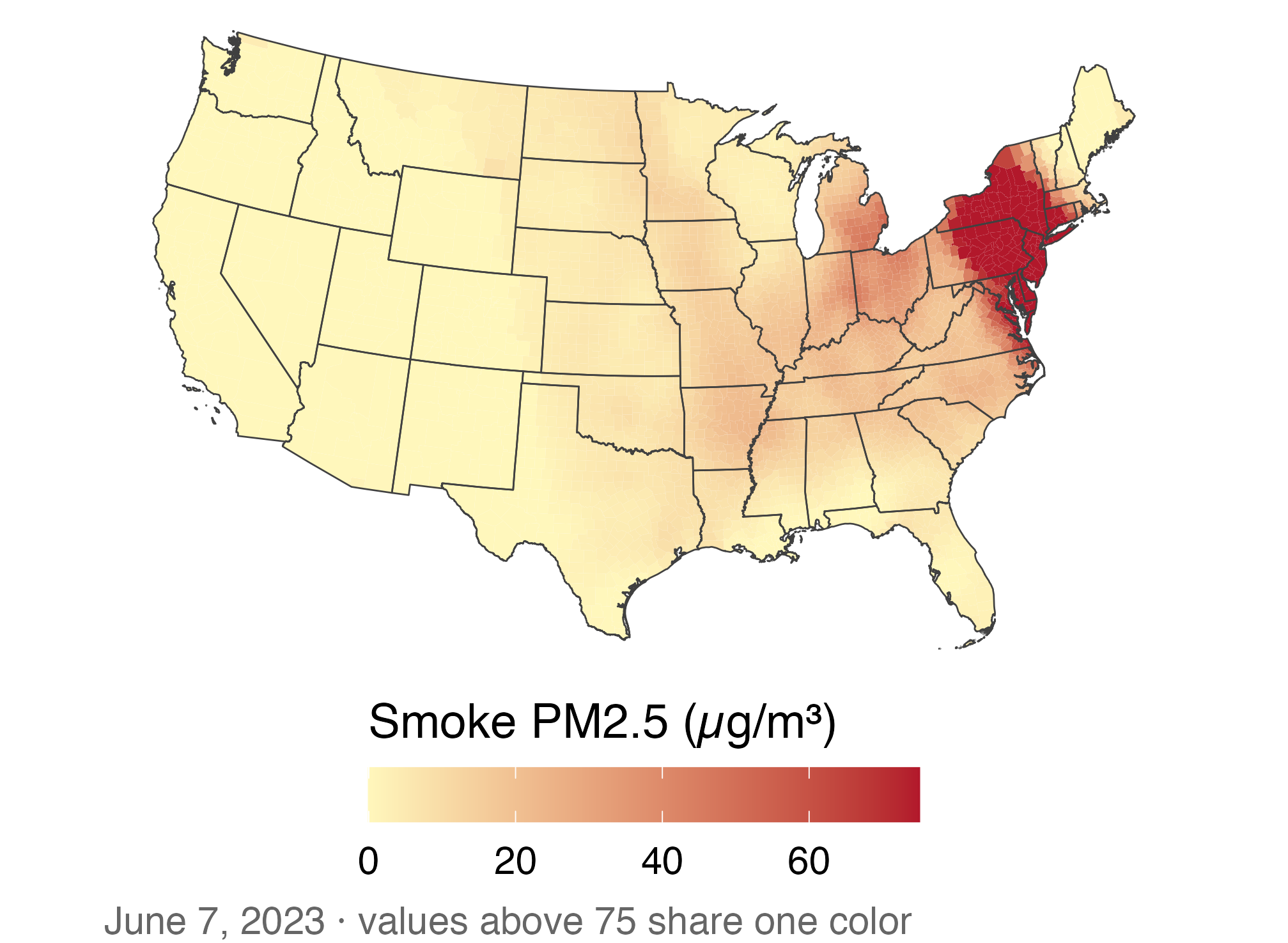
🚫 An extreme value stretches the gradient

p_smoke0 +
  scale_fill_gradient(
    low = "#fff7bc", high = "#b2182b",
    limits = c(0, 75), oob = squish,
    name = "Smoke PM2.5 (µg/m³)"
  ) +
  labs(caption = paste(
    "June 7, 2023 · values above 75",
    "share one color"
  ))

The same June 7 smoke map with the color scale capped at 75 micrograms per cubic meter. More Midwest and eastern variation appears, but all values above 75 share the darkest color.

  • Capping the scale reveals mid-range variation but hides differences above 75.
  • The next map uses labeled bins so readers can see the cutoffs.

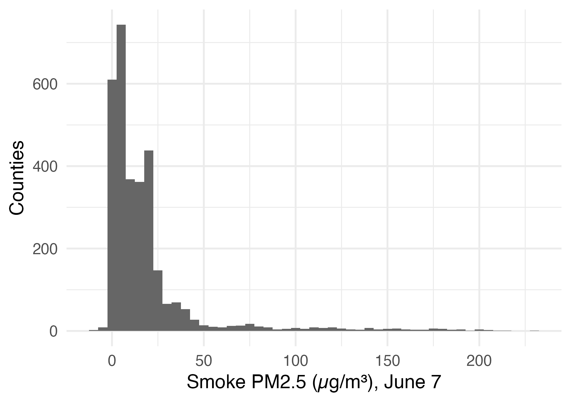
📊 Most counties sit at the bottom of the scale

ggplot(june7, aes(x = smoke_pm25)) +
  geom_histogram(binwidth = 5,
                 fill = "grey40") +
  theme_minimal(base_size = 13) +
  labs(x = "Smoke PM2.5 (µg/m³), June 7",
       y = "Counties")

Histogram of June 7 county smoke PM2.5; most counties have low values, with a long right tail above 200 micrograms per cubic meter.

  • Median 9.7, maximum 229 µg/m³: a long right tail.
  • A few small negatives come from subtracting the background from a noisy total: measurement noise, not “negative smoke.”

🎨 Bin the scale at meaningful breaks

pm25_bins <- scale_fill_fermenter(
  palette = "YlOrRd", direction = 1,
  breaks = c(5, 15, 35, 75, 150),
  name = "PM2.5 (µg/m³)"
)

ggplot(smoke_june7) +
  geom_sf(aes(fill = smoke_pm25),
          color = NA) +
  state_lines + pm25_bins + us_albers +
  labs(caption =
    "Smoke PM2.5, June 7, 2023 · CSU")

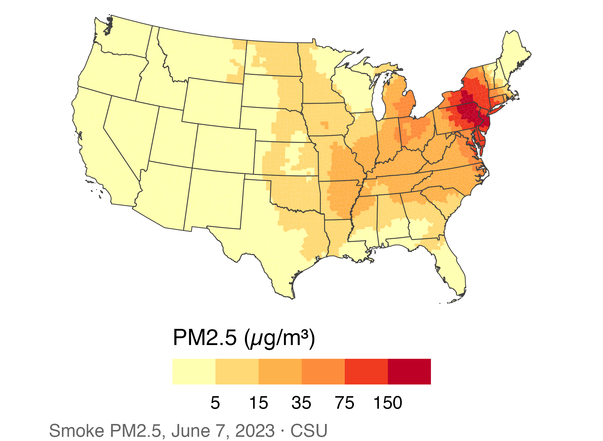
June 7 county smoke PM2.5 in bins at 5, 15, 35, 75, and 150 micrograms per cubic meter; the highest bins cluster in the Northeast.

  • 35 µg/m³ is the level of EPA’s 24-hour standard for total PM2.5; here it is only a reference for the smoke part. Negatives fall in the lowest bin.
  • We save the scale as pm25_bins and reuse it for every PM2.5 map.

🔄 Different bins, different story

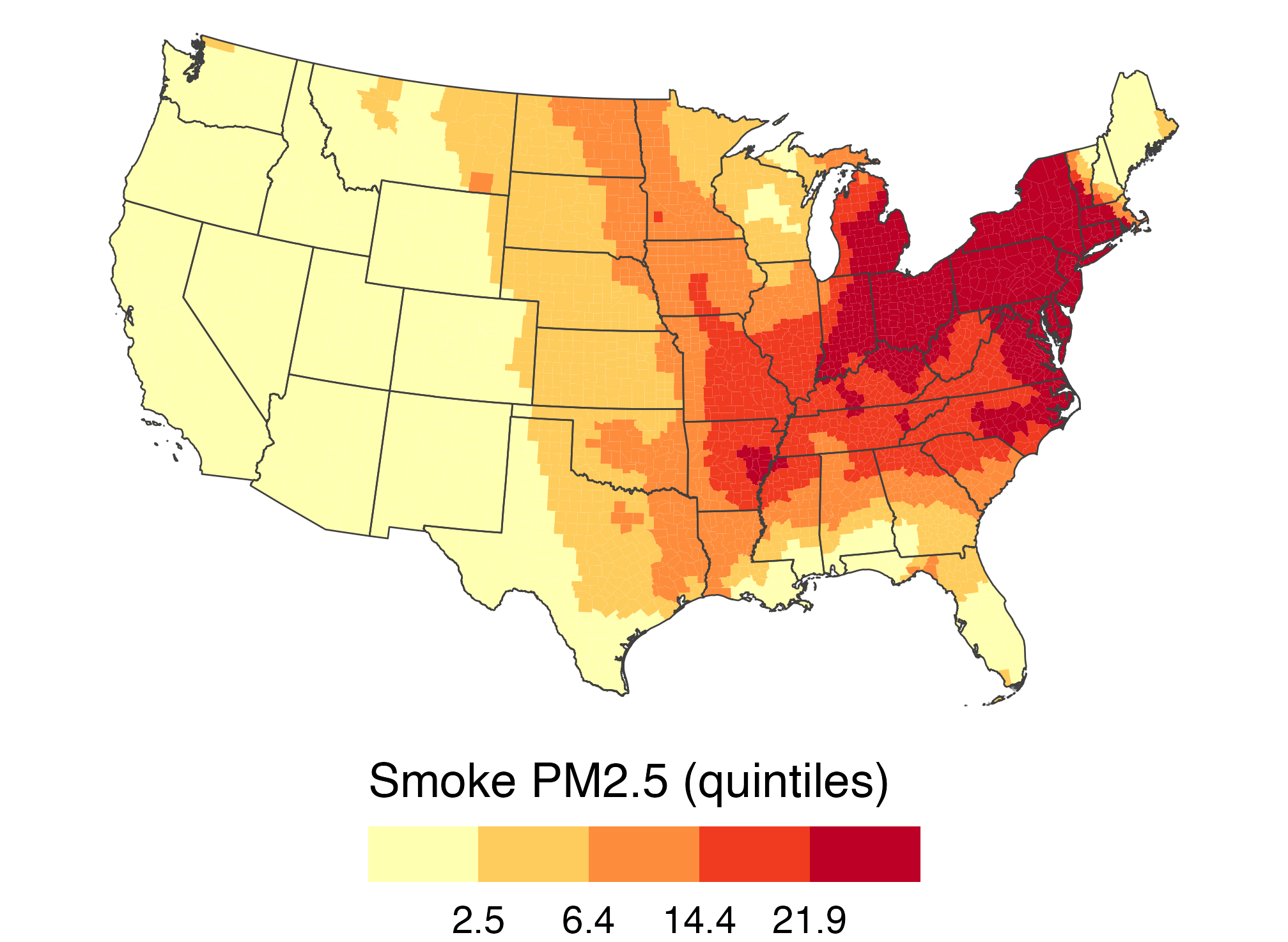
q_breaks <- quantile(june7$smoke_pm25,
                     c(0.2, 0.4, 0.6, 0.8))

ggplot(smoke_june7) +
  geom_sf(aes(fill = smoke_pm25),
          color = NA) +
  state_lines + us_albers +
  scale_fill_fermenter(
    palette = "YlOrRd", direction = 1,
    breaks = q_breaks,
    labels = label_number(0.1),
    name = "Smoke PM2.5 (quintiles)"
  )

The same June 7 county smoke mapped by quintiles; colors are spread more evenly across counties than on the fixed-break map.

Quintiles always put 40% of counties in the top two bins. Was 40% of the country smoky?

↔︎️ A diverging scale needs a meaningful midpoint

june_diff <- smoke_month |>
  filter(month == 6) |>
  group_by(GEOID) |>
  summarize(diff = smoke_pm25[year == 2023] -
    mean(smoke_pm25[year <= 2022]))

counties |>
  left_join(june_diff, by = "GEOID") |>
  ggplot(aes(fill = diff)) +
  geom_sf(color = NA) + state_lines +
  scale_fill_gradient2(midpoint = 0,
    low = "#2166ac", high = "#b2182b",
    name = "Change vs. usual June (µg/m³)") +
  us_albers

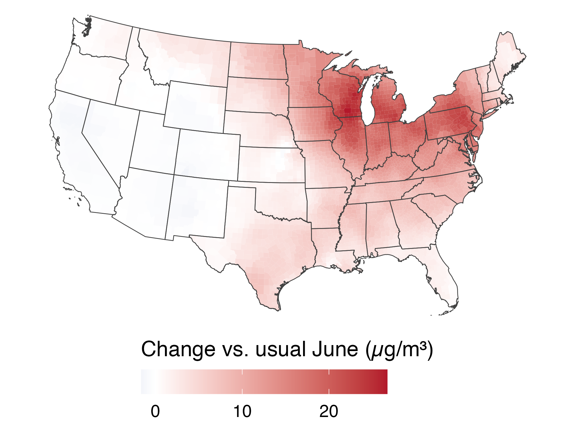
Difference between June 2023 smoke and a usual June; red increases cover much of the Midwest and East, while the West is near zero.

  • White (0) means “a typical June”: the West was near normal; the East far above.

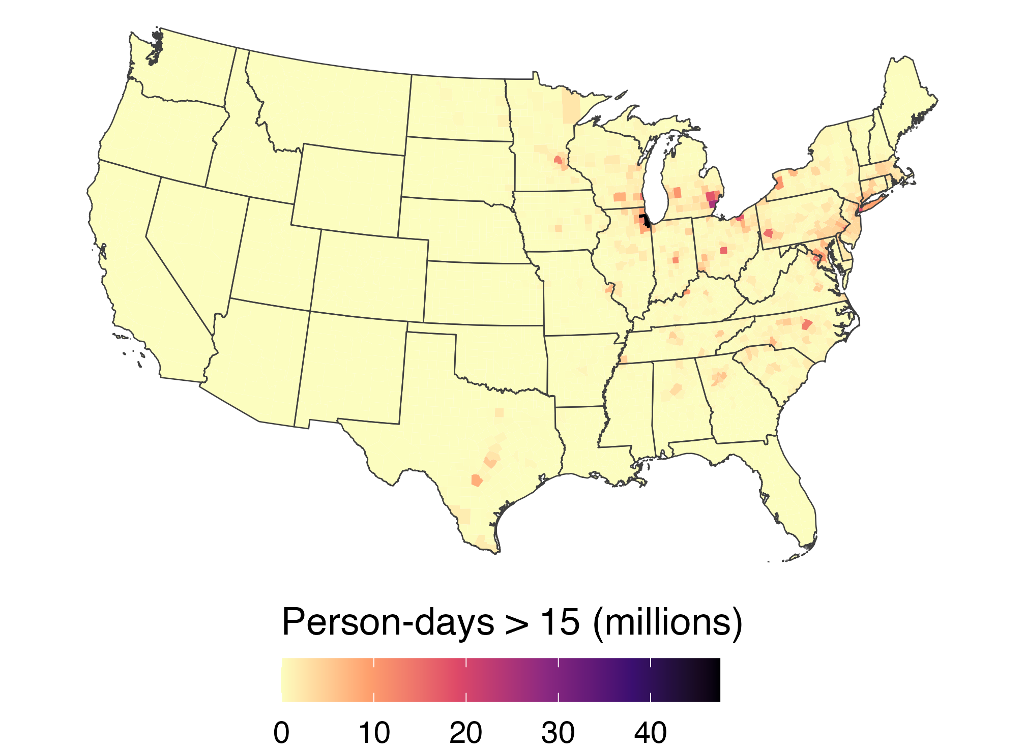
⚖️ Counts vs. rates: smoky days

june23 <- smoke_month |>
  filter(year == 2023, month == 6)

days_map <- counties |>
  left_join(june23, by = "GEOID") |>
  mutate(person_days = days_gt15 * pop_2020)

ggplot(days_map, aes(fill = days_gt15)) +
  geom_sf(color = NA) + state_lines +
  scale_fill_viridis_c(option = "magma",
    direction = -1,
    name = "Days with smoke > 15 µg/m³") +
  us_albers

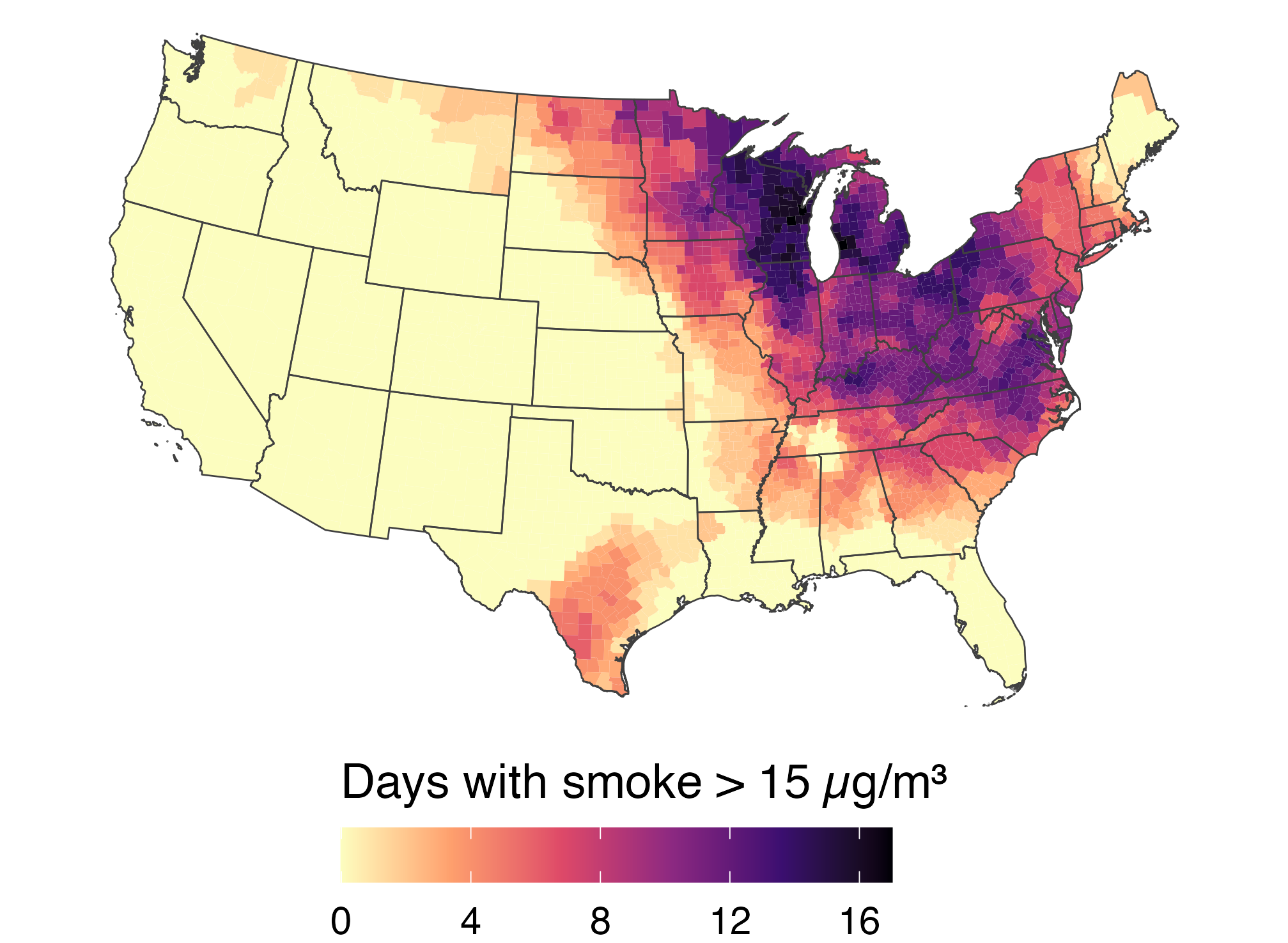
Number of June 2023 days with county smoke above 15 micrograms per cubic meter; the Midwest and East have the most days.

  • Rate: days_gt15 = smoky days for a typical resident, so small and large counties compare fairly. Up to 17 days (Michigan, Wisconsin).
  • Count: person_days = days × population, a total (next slide).

🏙️ Inside the smoke, totals follow population

ggplot(days_map,
       aes(fill = person_days / 1e6)) +
  geom_sf(color = NA) + state_lines +
  scale_fill_viridis_c(option = "magma",
    direction = -1,
    name = "Person-days > 15 (millions)") +
  us_albers

June 2023 person-days above 15 micrograms per cubic meter by county; high totals appear in populous eastern and Midwestern counties.

  • Big cities light up wherever smoke reached: Healy’s ur-choropleth.
  • 9 of the 10 darkest counties are among the 50 most populous; smoke-free Los Angeles stays pale.

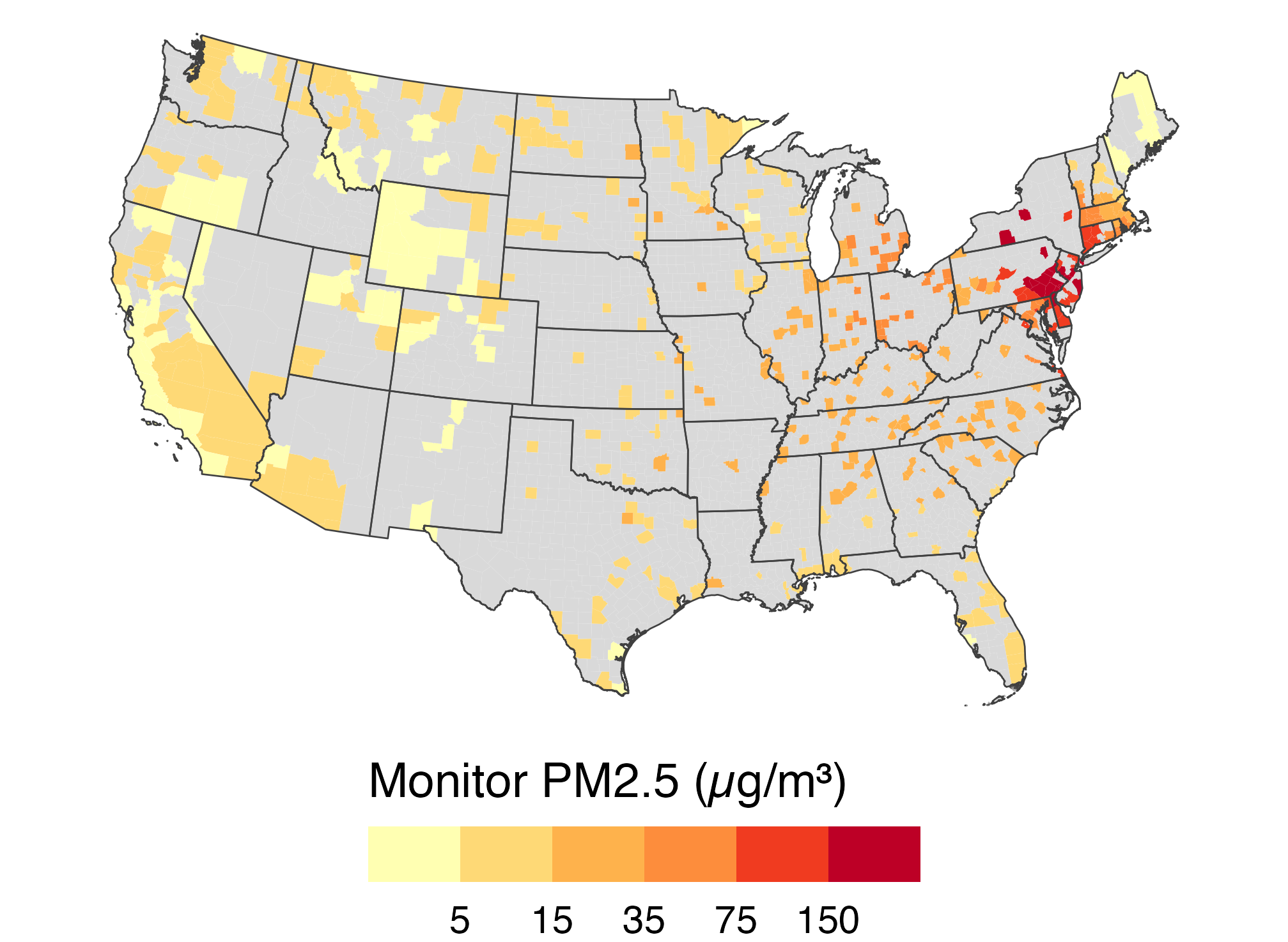
❔ Missing is not zero

monitor_june7 <- aqs |>
  filter(date == as.Date("2023-06-07")) |>
  group_by(GEOID) |>
  summarize(pm25 = mean(pm25))

counties |>
  left_join(monitor_june7, by = "GEOID") |>
  ggplot(aes(fill = pm25)) +
  geom_sf(color = NA) + state_lines +
  scale_fill_fermenter(palette = "YlOrRd",
    direction = 1, na.value = "grey85",
    breaks = c(5, 15, 35, 75, 150),
    name = "Monitor PM2.5 (µg/m³)") +
  us_albers

County map of monitor PM2.5 on June 7; many counties are grey because they have no monitor, while high observed values cluster in the Northeast.

  • Only 506 of 3,108 counties had a monitor reporting. Grey means no data, not clean air.

📅 Small-Multiple Maps

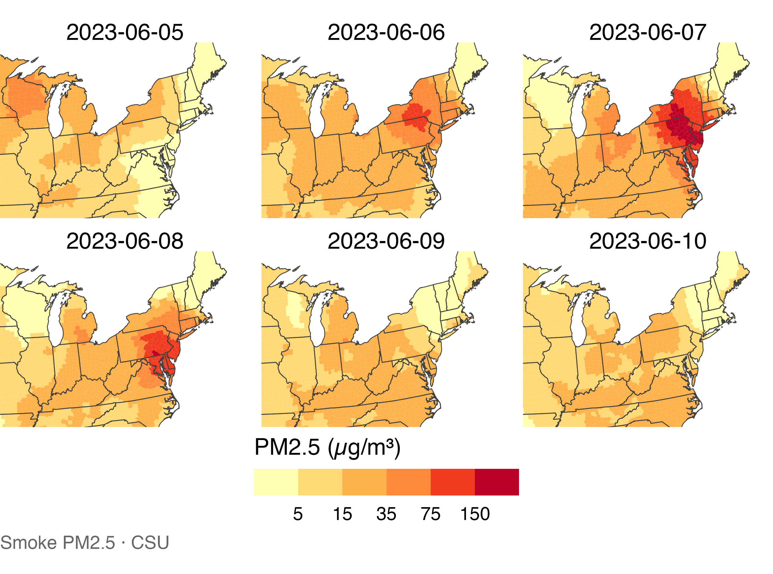
📅 Small multiples by day

days_5_10 <- smoke_day |>
  filter(between(date,
    as.Date("2023-06-05"),
    as.Date("2023-06-10")))

counties |>
  left_join(days_5_10,
            by = "GEOID") |>
  ggplot(aes(fill = smoke_pm25)) +
  geom_sf(color = NA) +
  state_lines +
  pm25_bins +
  facet_wrap(~ date, ncol = 3) +
  labs(caption =
    "Smoke PM2.5 · CSU") +
  coord_sf(crs = "ESRI:102003",
    xlim = c(-92, -67),
    ylim = c(35, 48),
    default_crs = st_crs(4326))

Six maps from June 5 through 10 share one smoke scale; the darkest area moves from New York and Pennsylvania toward the Mid-Atlantic.

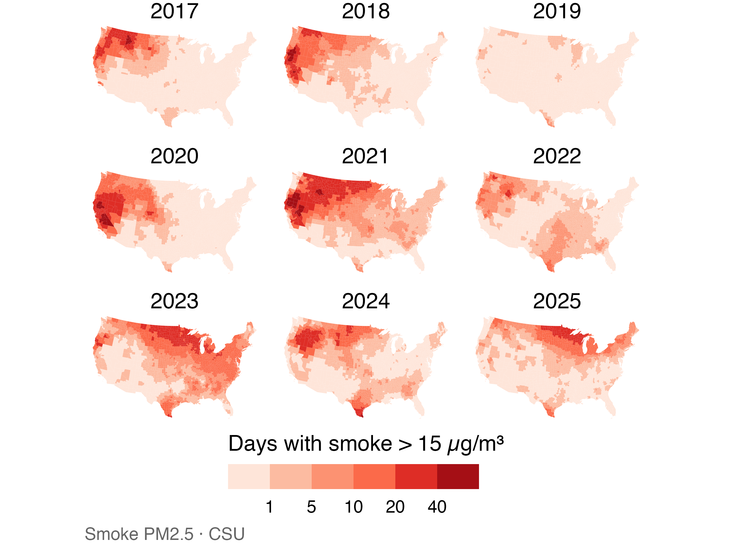
🗂️ Small multiples by year

yearly_days <- smoke_month |>
  filter(year >= 2017) |>
  summarize(days = sum(days_gt15),
            .by = c(GEOID, year))

counties |>
  left_join(yearly_days,
            by = "GEOID") |>
  ggplot(aes(fill = days)) +
  geom_sf(color = NA) +
  scale_fill_fermenter(
    palette = "Reds",
    direction = 1,
    breaks = c(1, 5, 10, 20, 40),
    name = paste(
      "Days with smoke > 15",
      "µg/m³"
    )) +
  facet_wrap(~ year, ncol = 3) +
  labs(caption =
    "Smoke PM2.5 · CSU") +
  us_albers

Nine annual maps for 2017 through 2025 share one scale for days above 15; smoke is prominent in the West in 2020 and 2021 and the East in 2023.

⚠️ Cautions for small-multiple maps

  • Keep one shared scale across panels (the facet_wrap() default).
  • Each panel is small, so fine detail disappears.
  • Big, sparsely populated western counties dominate the eye.
  • To compare timing in a few places, a line chart often works better.

Statebins draw every state as a same-sized tile; cartograms can resize states by population. Both make small, crowded states more visible while changing their geographic shapes or positions (Healy).

🔷 Hexbin Maps

🔷 A regular grid changes the map’s units

  • County boundaries vary greatly in size. A hex grid uses cells of equal area.
  • The map still preserves location and neighboring cells.
  • We assign each county to the cell containing a point inside its boundary.

📐 Build an sf hex grid

states_m <- st_transform(states, 5070)
hex_geom <- st_make_grid(
  states_m, cellsize = 180000,
  square = FALSE
)
hex_grid <- st_sf(
  hex_id = seq_along(hex_geom),
  geometry = hex_geom
)
  • EPSG:5070 lets us set the grid spacing to 180 km.
  • The grid consists of equal-area cells in this projection.

📍 Assign counties to hexagons

county_points <- smoke_june7 |>
  st_transform(5070) |>
  st_point_on_surface()

hex_counties <- county_points |>
  select(GEOID, smoke_pm25, pop_2020) |>
  st_join(hex_grid |> select(hex_id),
          join = st_within)
  • st_point_on_surface() puts one representative point inside each county.
  • st_join() assigns that point to one hexagon.

🔥 Summarize smoke within hexagons

hex_summary <- hex_counties |>
  st_drop_geometry() |>
  filter(!is.na(hex_id)) |>
  summarize(
    smoke_pm25 = weighted.mean(
      smoke_pm25, pop_2020
    ),
    counties = n(), .by = hex_id
  )

hex_smoke <- hex_grid |>
  left_join(hex_summary, by = "hex_id") |>
  filter(!is.na(smoke_pm25))
  • Each cell summarizes its assigned counties using population weights.
  • A county is represented in one cell, even when its area spans several cells.

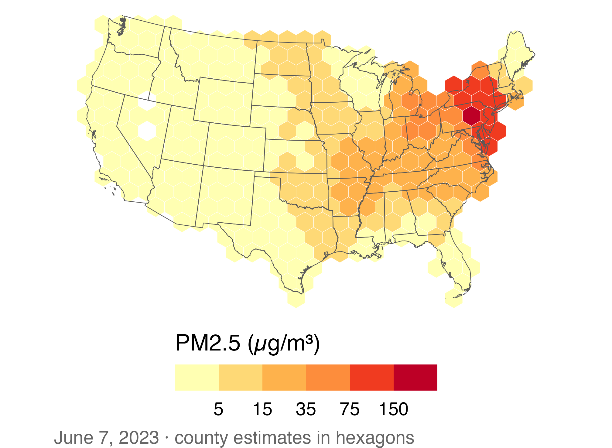
🔥 Fill hexagons with smoke estimates

ggplot(hex_smoke) +
  geom_sf(aes(fill = smoke_pm25),
          color = "white",
          linewidth = 0.1) +
  geom_sf(data = states_m, fill = NA,
          color = "grey35",
          linewidth = 0.2) +
  pm25_bins + us_albers +
  labs(caption = paste(
    "June 7, 2023 · county estimates",
    "in hexagons"
  ))

Equal-area hexagons replace county polygons on a June 7 smoke map. The darkest cells cluster in the Northeast, and state outlines remain visible.

  • The same county estimates now appear in regular spatial units.
  • State outlines give viewers a geographic reference.

⚖️ Hexagons and counties answer different questions

  • County maps match the units in the source table and show local boundaries.
  • Hexagons make area sizes consistent but discard county shapes.
  • Neither map identifies the concentration that each person actually inhaled.

🔁 Plotting Multiple Layers

📂 Read the fire and plume layers

fires <- read_csv(
  paste0(course_url, "wildfire_firms_canada_2023.csv"),
  col_types = cols(acq_time = col_character()))
nbac <- read_sf(paste0(course_url, "wildfire_nbac_burned_area_2023.geojson"))
plumes <- read_sf(paste0(course_url, "wildfire_hms_smoke_2023_06.geojson"))
  • fires: one row per satellite fire detection (latitude, longitude, fire power).
  • nbac: one outer outline per 2023 fire; plumes: one smoke plume per row.
  • The outlines fill in unburned islands, so for burned area use area_ha, not st_area(): 14.8 vs. 16.9 million ha.

📍 Fire detections become points

firms_sf <- fires |>
  st_as_sf(coords = c("longitude", "latitude"), crs = 4326)

firms_sf |>
  select(local_date, frp, prov_abbr) |>
  print(n = 3)
Simple feature collection with 280457 features and 3 fields
Geometry type: POINT
Dimension:     XY
Bounding box:  xmin: -140.7173 ymin: 42.102 xmax: -55.498 ymax: 81.8968
Geodetic CRS:  WGS 84
# A tibble: 280,457 × 4
  local_date   frp prov_abbr            geometry
  <date>     <dbl> <chr>             <POINT [°]>
1 2023-01-02     0 AB        (-117.9582 53.4929)
2 2023-01-02     0 AB        (-117.9781 53.4971)
3 2023-01-02     0 AB        (-117.9604 53.4998)
# ℹ 280,454 more rows
  • coords: x (longitude) first, then y (latitude). crs = 4326: the numbers are degrees.

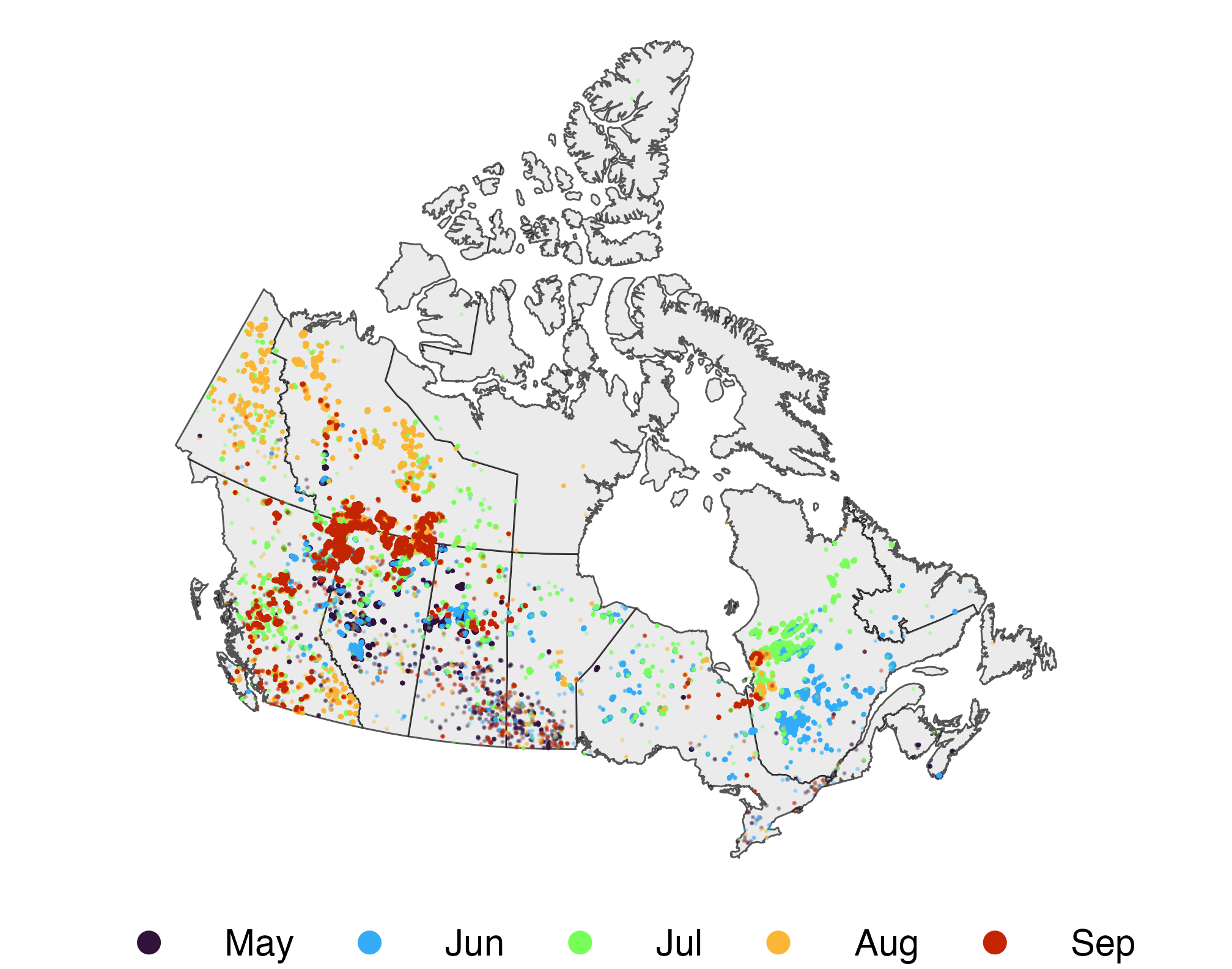
🔥 The 2023 fire season

fires_season <- firms_sf |>
  filter(month(local_date) %in% 5:9) |>
  mutate(month = month(local_date,
                       label = TRUE))

ggplot() +
  geom_sf(data = provinces, fill = "grey92") +
  geom_sf(data = fires_season, size = 0.05,
          aes(color = month), alpha = 0.3) +
  scale_color_viridis_d(
    option = "turbo", end = 0.9
  ) +
  guides(color = guide_legend(override.aes =
    list(size = 3, alpha = 1))) +
  na_lcc + labs(color = NULL)

Canadian fire detections from May through September 2023, colored by month; detections cluster across western Canada and parts of Quebec.

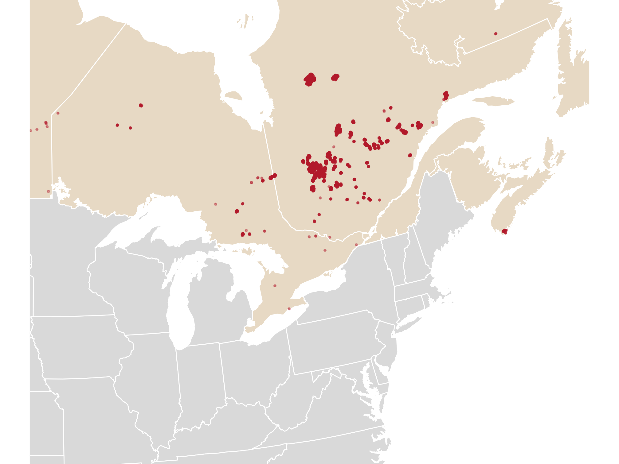
📅 One week: June 1–7

fires_week <- firms_sf |>
  filter(between(local_date,
    as.Date("2023-06-01"),
    as.Date("2023-06-07")))

ggplot() +
  geom_sf(data = provinces,
          fill = "#e7d9c4", color = "white") +
  geom_sf(data = states,
          fill = "grey85", color = "white") +
  geom_sf(data = fires_week, size = 0.3,
          color = "#b2182b", alpha = 0.4) +
  east_zoom

Fire detections from June 1 through 7 cluster in Quebec on a map of eastern Canada and the northeastern United States.

  • Quebec had 5,619 detections in these seven days, more than any other province.

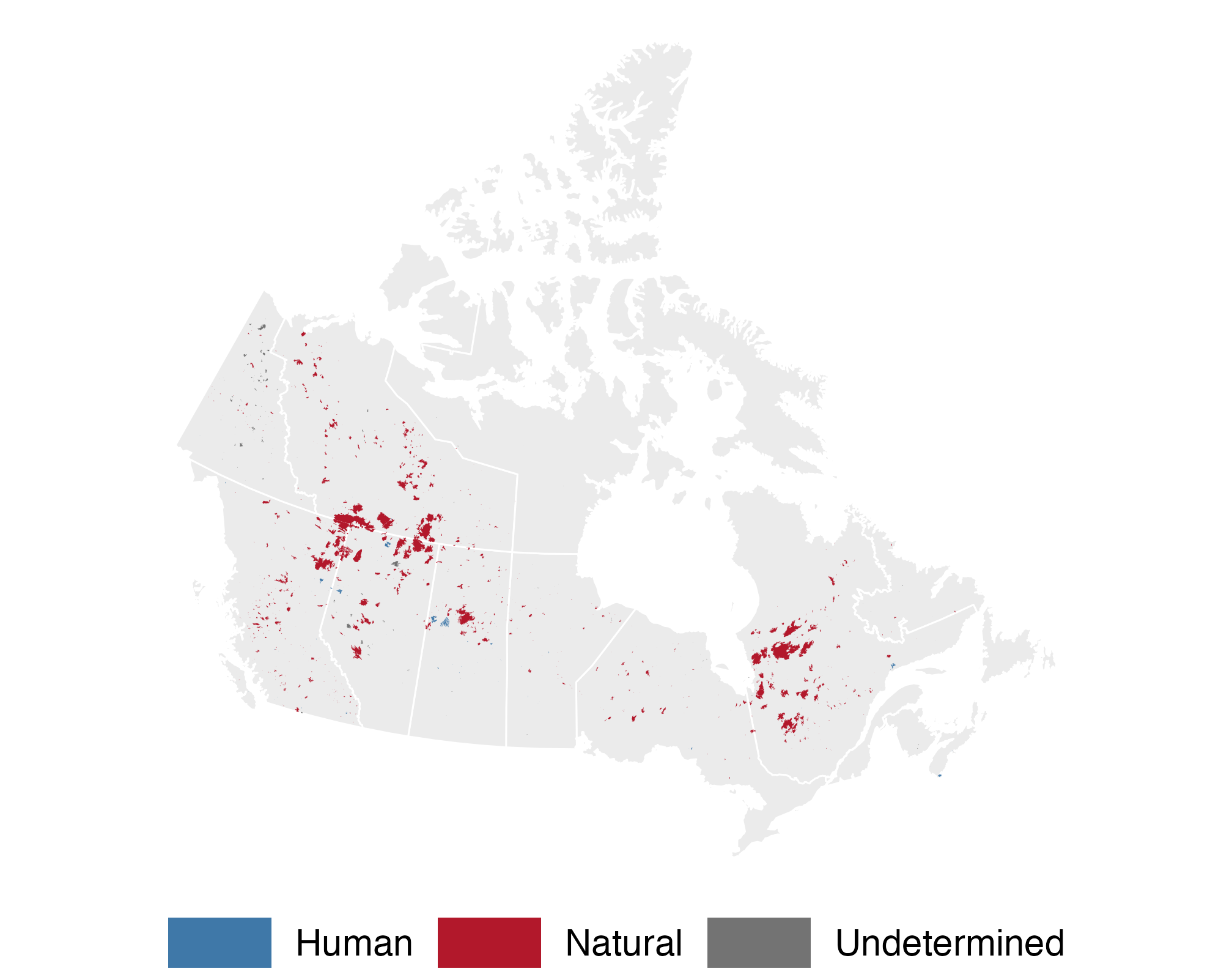
🟫 Burned-area perimeters are polygons

ggplot() +
  geom_sf(data = provinces,
          fill = "grey92", color = "white") +
  geom_sf(data = nbac, aes(fill = cause),
          color = NA) +
  scale_fill_manual(values = c(
    Human = "#3f78a8",
    Natural = "#b2182b",
    Undetermined = "grey45")) +
  na_lcc + labs(fill = NULL)

2023 Canadian burned-area perimeters, colored by cause, concentrated in western provinces and Quebec.

  • 755 of 968 mapped fires had a natural cause (mostly lightning).

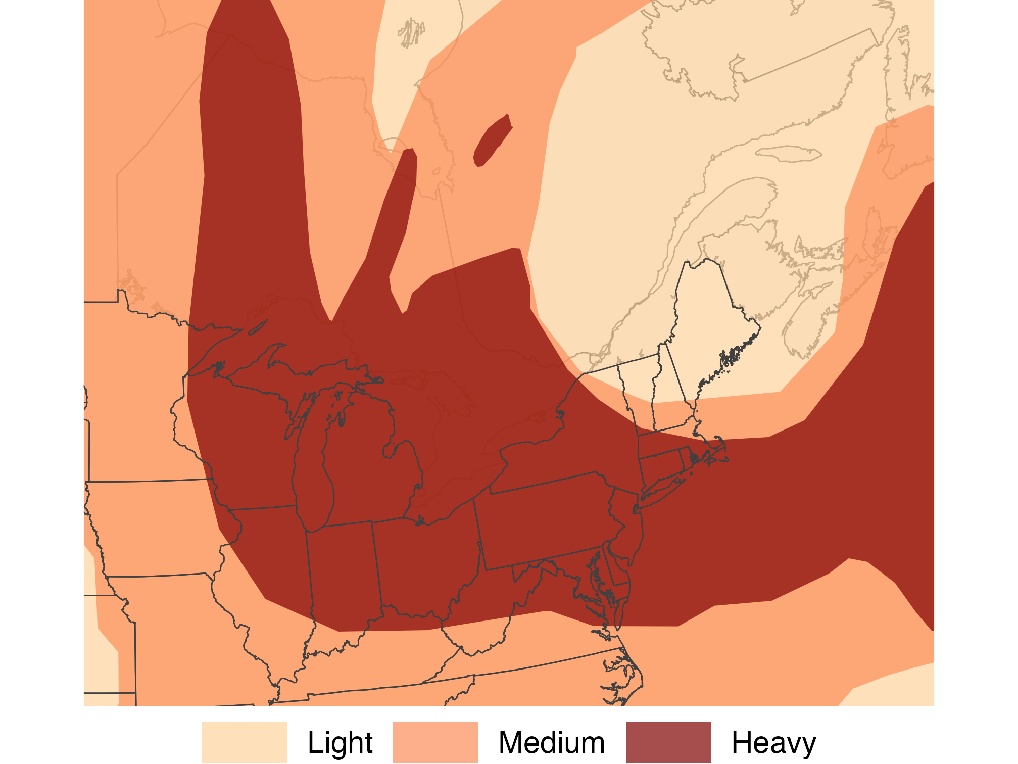
🌫️ Smoke plumes are overlapping polygons

plumes_june7 <- plumes |>
  filter(date == as.Date("2023-06-07")) |>
  mutate(density = factor(density, levels =
    c("Light", "Medium", "Heavy")))
plumes_by_density <- plumes_june7 |>
  group_by(density) |> summarize()

ggplot() +
  geom_sf(data = provinces, fill = "grey96") +
  geom_sf(data = plumes_by_density, color = NA,
          aes(fill = density), alpha = 0.7) +
  state_lines + scale_fill_manual(values = c(
    "#fdd49e", "#fc8d59", "#7f0000")) +
  east_zoom + labs(fill = NULL)

June 7 satellite smoke plume polygons cover much of eastern North America; Heavy plumes span the Great Lakes and Mid-Atlantic.

  • group_by(density) |> summarize() merges overlapping plumes, so each color is one density level.

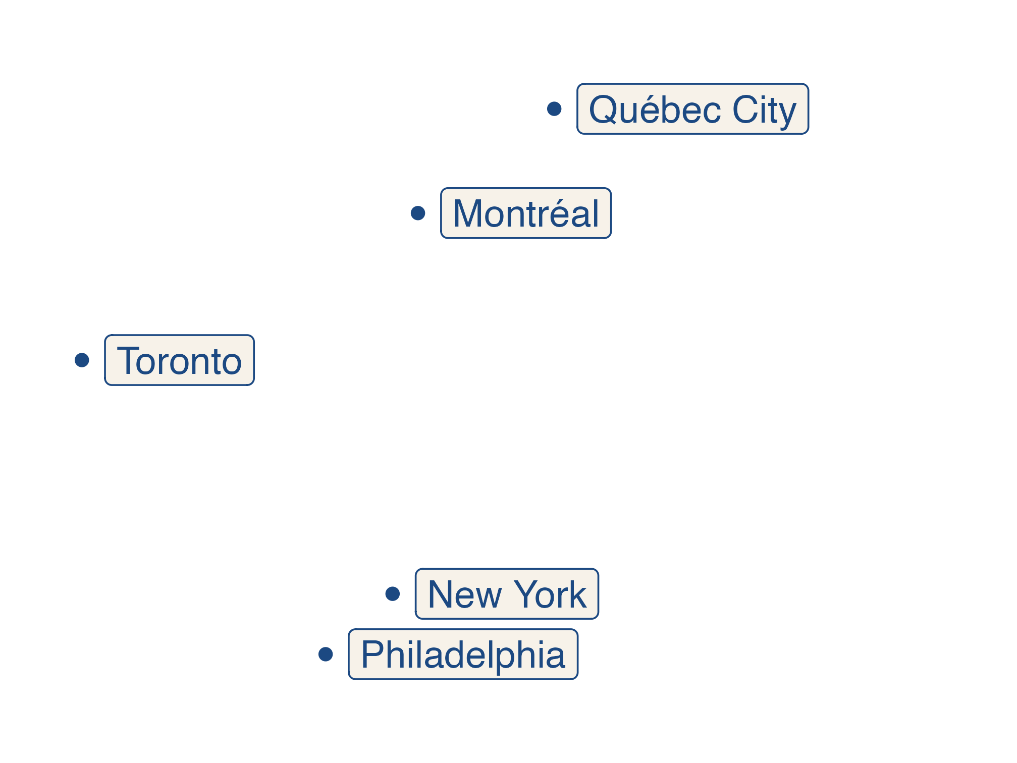
✏️ Make your own points: cities

cities <- tribble(
  ~city,          ~lat,    ~lon,
  "New York",     40.713, -74.006,
  "Philadelphia", 39.953, -75.165,
  "Montréal",     45.502, -73.567,
  "Toronto",      43.653, -79.383,
  "Québec City",  46.814, -71.208
) |>
  st_as_sf(coords = c("lon", "lat"),
           crs = 4326)
ggplot(cities) +
  geom_sf(color = "#1c4982", size = 2) +
  geom_sf_label(aes(label = city),
    color = "#1c4982", fill = "#f7f2e9",
    hjust = 0, nudge_x = 0.4) +
  coord_sf(xlim = c(-80, -64))

Five labeled points locate Toronto, Montréal, Québec City, New York, and Philadelphia relative to one another.

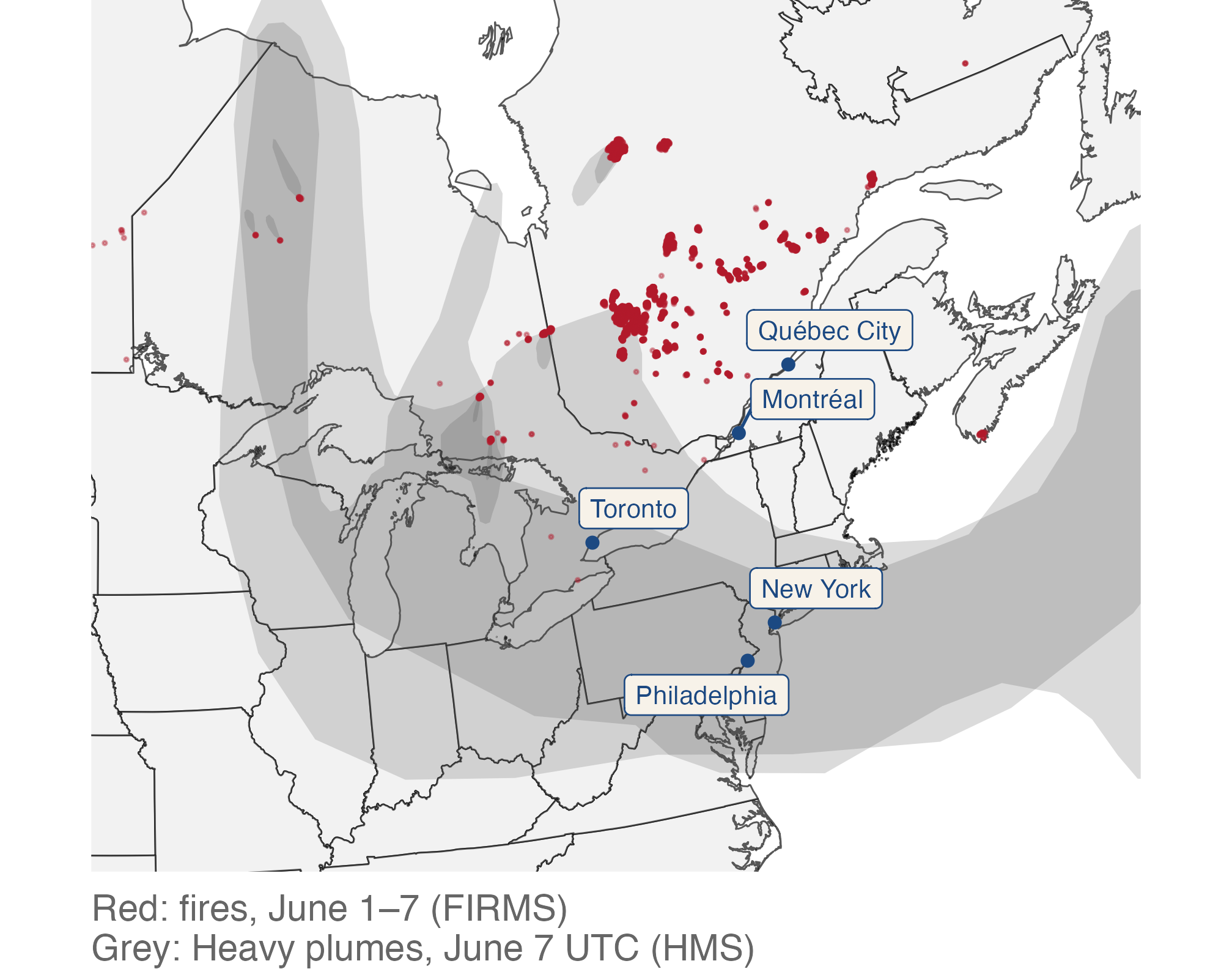
🔁 Fire → wind → smoke: put the layers together

heavy_june7 <- plumes_june7 |>
  filter(density == "Heavy")

ggplot() +
  geom_sf(data = provinces, fill = "grey95") +
  geom_sf(data = states, fill = "grey95") +
  geom_sf(data = heavy_june7, color = NA,
          fill = "grey30", alpha = 0.2) +
  geom_sf(data = fires_week, size = 0.3,
          color = "#b2182b", alpha = 0.4) +
  geom_sf(data = cities, size = 1.5,
          color = "#1c4982") +
  geom_label_repel(
    data = cities, size = 3, seed = 42,
    aes(label = city, geometry = geometry),
    stat = "sf_coordinates",
    color = "#1c4982", fill = "#f7f2e9"
  ) + east_zoom +
  labs(caption = paste0(
    "Red: fires, June 1–7 (FIRMS)\n",
    "Grey: Heavy plumes, June 7 UTC (HMS)"
  ))

Fire detections cluster in Quebec; translucent Heavy plumes extend south over labeled cities from Toronto to Philadelphia.

  • geom_label_repel(stat = "sf_coordinates") works like geom_sf_label() but pushes labels apart.

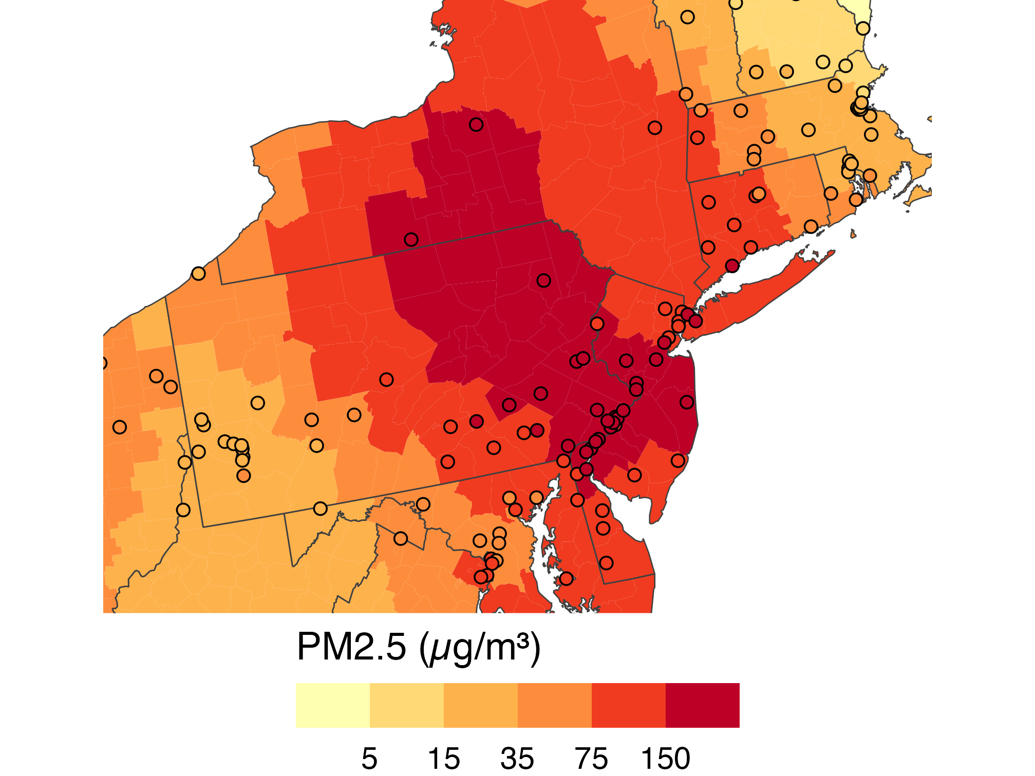
📍 Monitors and counties share one scale

monitors_june7 <- aqs |>
  filter(date == as.Date("2023-06-07")) |>
  st_as_sf(coords = c("longitude",
    "latitude"), crs = 4326)

ggplot() +
  geom_sf(data = smoke_june7, color = NA,
          aes(fill = total_pm25)) +
  state_lines +
  geom_sf(data = monitors_june7, shape = 21,
          aes(fill = pm25), size = 2) +
  pm25_bins + coord_sf(crs = "ESRI:102003",
    xlim = c(-81, -71), ylim = c(38.5, 44),
    default_crs = st_crs(4326))

County estimates and air-monitor readings share one total PM2.5 scale around Pennsylvania, New Jersey, and New York; both show high values in the region.

  • Fill is total PM2.5 for both: county estimates and monitor readings.
  • Both layers map fill, so one binned scale colors counties and monitors alike.

🔗 Spatial Joins

🔎 Which counties touched a Heavy plume?

counties_heavy <- counties |>
  st_filter(heavy_june7)

ggplot() +
  geom_sf(data = counties_heavy,
          fill = "#b6533c", color = NA) +
  state_lines + us_albers

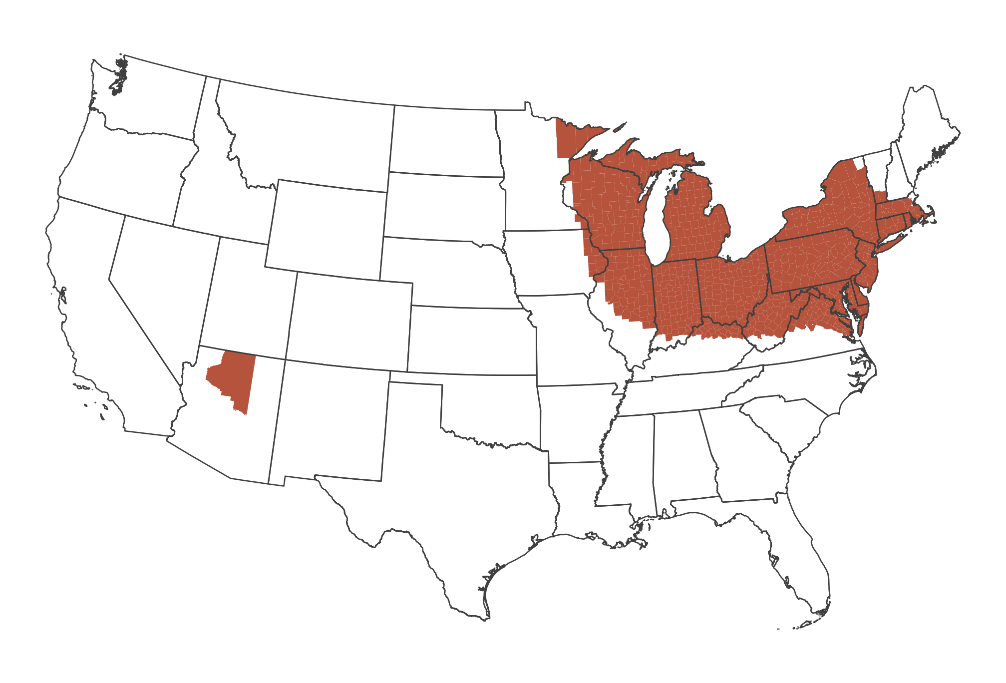
Counties intersecting a June 7 Heavy plume are highlighted, mainly across the Great Lakes and Northeast, with a smaller group in Arizona.

  • st_filter() keeps counties whose shapes intersect a Heavy plume (June 7, UTC).
  • nrow(counties_heavy): 721 counties touched, with 113.3 million residents in those counties.

🌫️ Plume outlines and surface estimates differ

exposure <- smoke_june7 |>
  mutate(
    touched = GEOID %in% counties_heavy$GEOID,
    group = case_when(
      touched & smoke_pm25 > 35 ~ "Both",
      touched ~ "Plume only",
      smoke_pm25 > 35 ~ "Surface > 35 only",
      TRUE ~ "Neither"))

ggplot(exposure, aes(fill = group)) +
  geom_sf(color = NA) + state_lines +
  scale_fill_manual(values = c(
    Both = "#7f2704", Neither = "grey90",
    "Plume only" = "#fdae6b",
    "Surface > 35 only" = "#3f78a8")) +
  guides(fill = guide_legend(nrow = 2,
    title = NULL)) + us_albers +
  labs(caption = paste0(
    "June 7, 2023. Plume: Heavy HMS plume\n",
    "(UTC date). Surface: smoke > 35 µg/m³"))

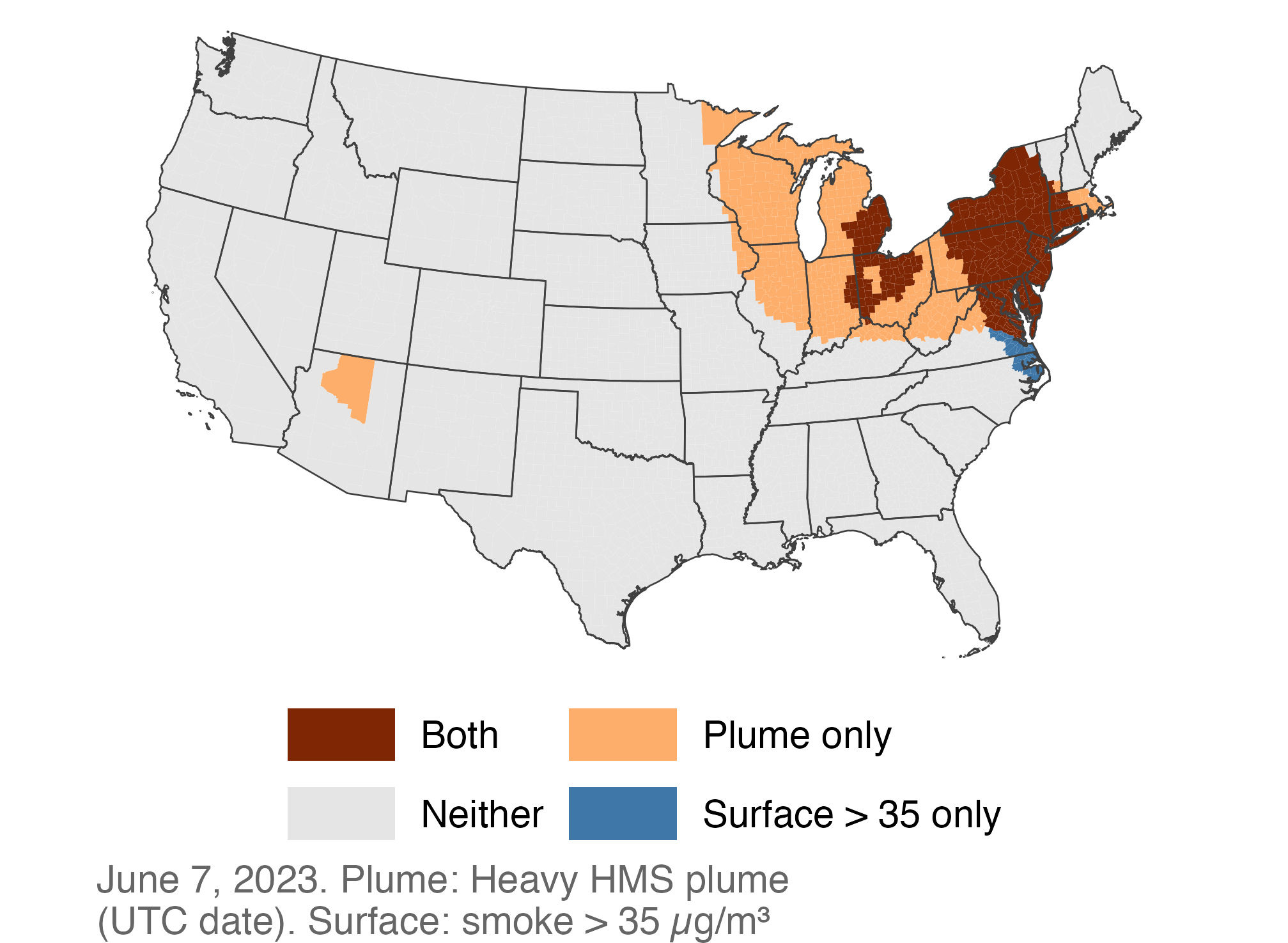
Counties classified by Heavy plume overlap and estimated surface smoke above 35; many northeastern counties meet both, while plume-only counties extend farther west.

👥 Count residents by county group

exposure |>
  st_drop_geometry() |>
  group_by(group) |>
  summarize(counties = n(),
            people_millions = sum(pop_2020) / 1e6)
# A tibble: 4 × 3
  group             counties people_millions
  <chr>                <int>           <dbl>
1 Both                   296           71.9 
2 Neither               2351          213.  
3 Plume only             425           41.4 
4 Surface > 35 only       36            2.89
  • st_drop_geometry(): a plain table, so summarize() won’t merge shapes.
  • Residents of plume-touched counties: 113.3 million. Residents of counties with estimated surface smoke > 35: 74.8 million.
  • Both are county-level indicators, not counts of what each resident inhaled.

📍 Points in polygons with st_join()

fires_prov <- firms_sf |>
  mutate(id = row_number()) |>
  st_join(provinces |> select(prov_join = prov_abbr))

c(detections = nrow(firms_sf), rows = nrow(fires_prov))
detections       rows 
    280457     280457 
  • st_join() returns one row for each point–polygon match. It adds the polygon’s columns to the point.
  • Same number of rows here: no detection matched two provinces. A point inside two overlapping polygons would get two rows, so compare nrow() before and after every join.

🔍 Check the join before you count

fires_prov |>
  st_drop_geometry() |>
  summarize(
    matches = sum(!is.na(prov_join)),
    .by = id) |>
  count(matches)
# A tibble: 2 × 2
  matches      n
    <int>  <int>
1       0     22
2       1 280435
join_check <- fires_prov |>
  st_drop_geometry() |>
  count(check = case_when(
    is.na(prov_join) ~ "outside",
    prov_join == prov_abbr ~ "same",
    TRUE ~ "different"))
join_check
# A tibble: 3 × 2
  check          n
  <chr>      <int>
1 different    236
2 outside       22
3 same      280199
  • matches: 0 = outside every polygon, 1 = one province. No 2s, so each row is one detection.
  • check: does the polygon agree with the label prov_abbr? The few misses sit on borders and coasts.

📊 Count points per polygon, then map the counts

fire_counts <- fires_prov |>
  st_drop_geometry() |>
  count(prov_join, name = "detections")

provinces |>
  left_join(fire_counts,
    by = c("prov_abbr" = "prov_join")) |>
  mutate(detections =
    replace_na(detections, 0)) |>
  ggplot(aes(fill = detections)) +
  geom_sf(color = "white") +
  scale_fill_viridis_c(
    option = "inferno", labels = comma,
    name = "Fire detections, 2023"
  ) +
  na_lcc

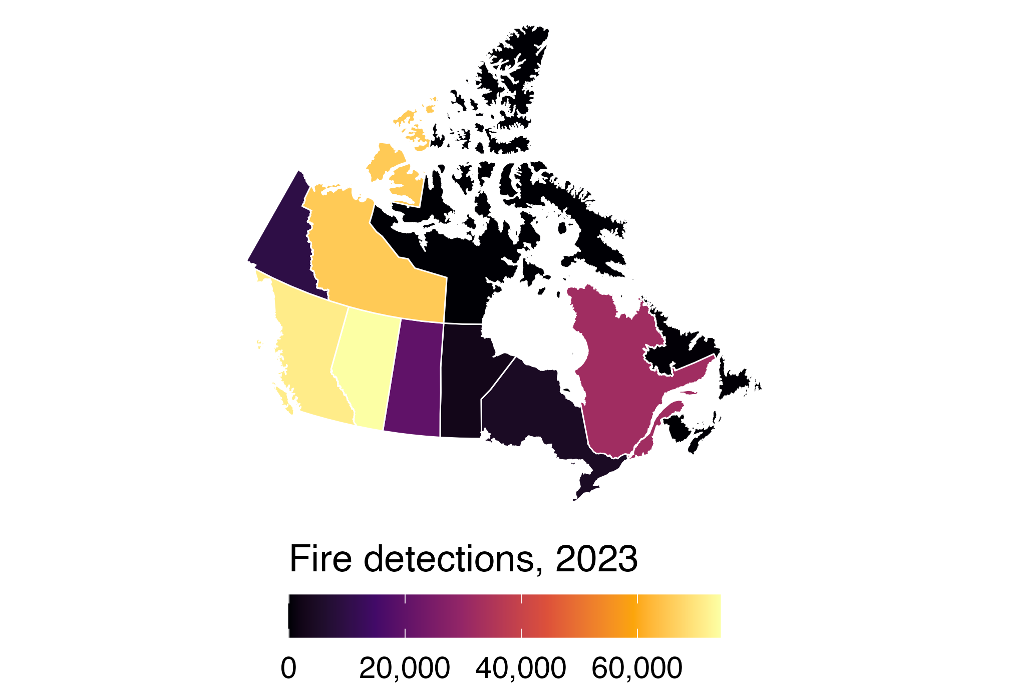
Canadian provinces colored by 2023 fire-detection counts; Alberta has the most, followed by British Columbia and the Northwest Territories, while Nunavut is near the low end of the scale.

  • Here NA means no detections: a true zero (Prince Edward Island).

Nunavut is three times Alberta’s size but had 50 detections. Counts or detections per km²?

⚖️ From counties to states with population weights

state_june7 <- smoke_june7 |>
  st_drop_geometry() |>
  group_by(STUSPS) |>
  summarize(smoke = weighted.mean(
    smoke_pm25, pop_2020))

states |>
  left_join(state_june7, by = "STUSPS") |>
  ggplot(aes(fill = smoke)) +
  geom_sf(color = "white",
          linewidth = 0.2) +
  pm25_bins + us_albers +
  labs(caption = "Smoke PM2.5, June 7, 2023")

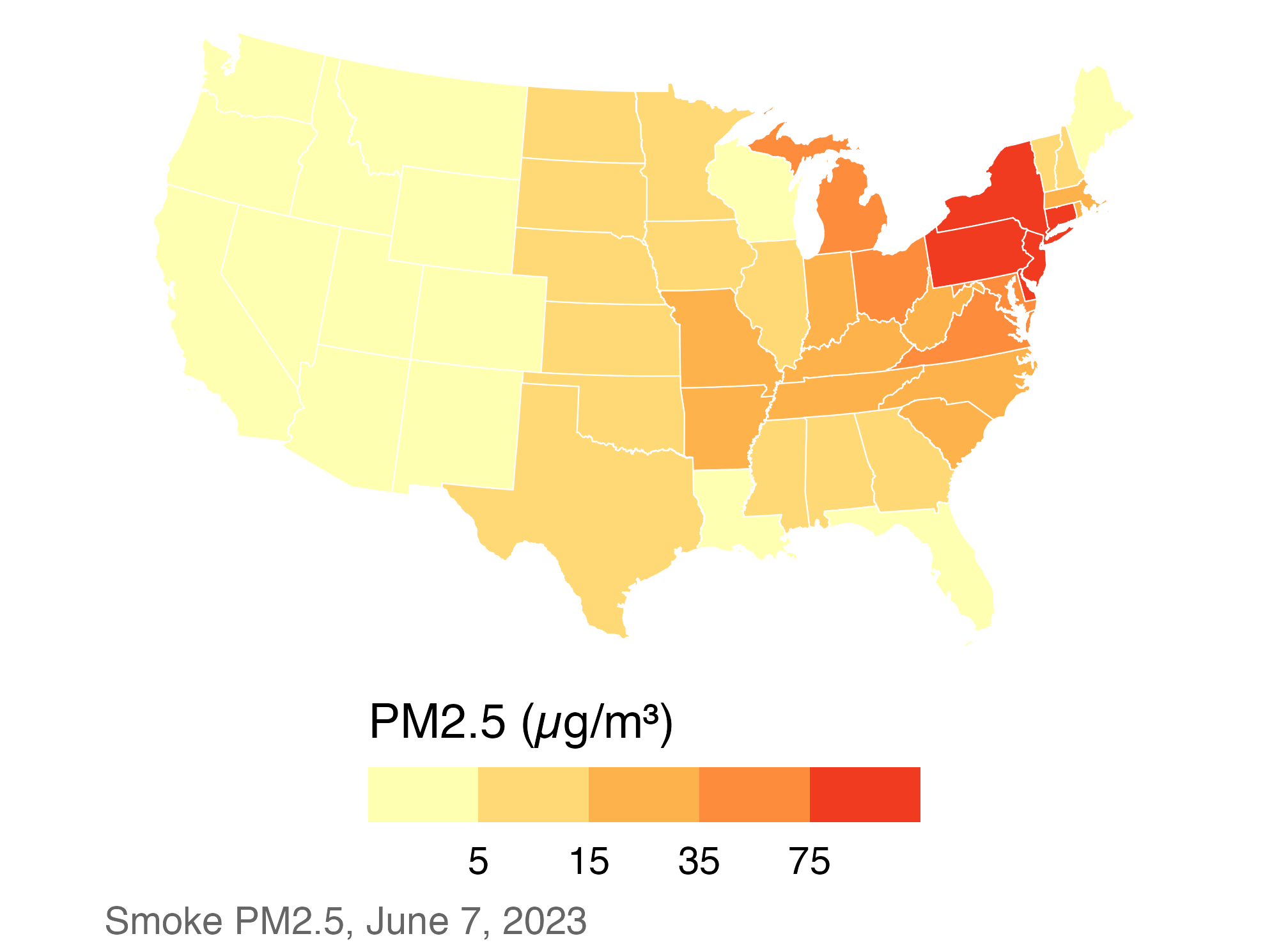
Population-weighted state smoke PM2.5 on June 7; New Jersey, Pennsylvania, Delaware, and New York are highest while western states are low.

  • Weighting by population gives the smoke level of the average resident.

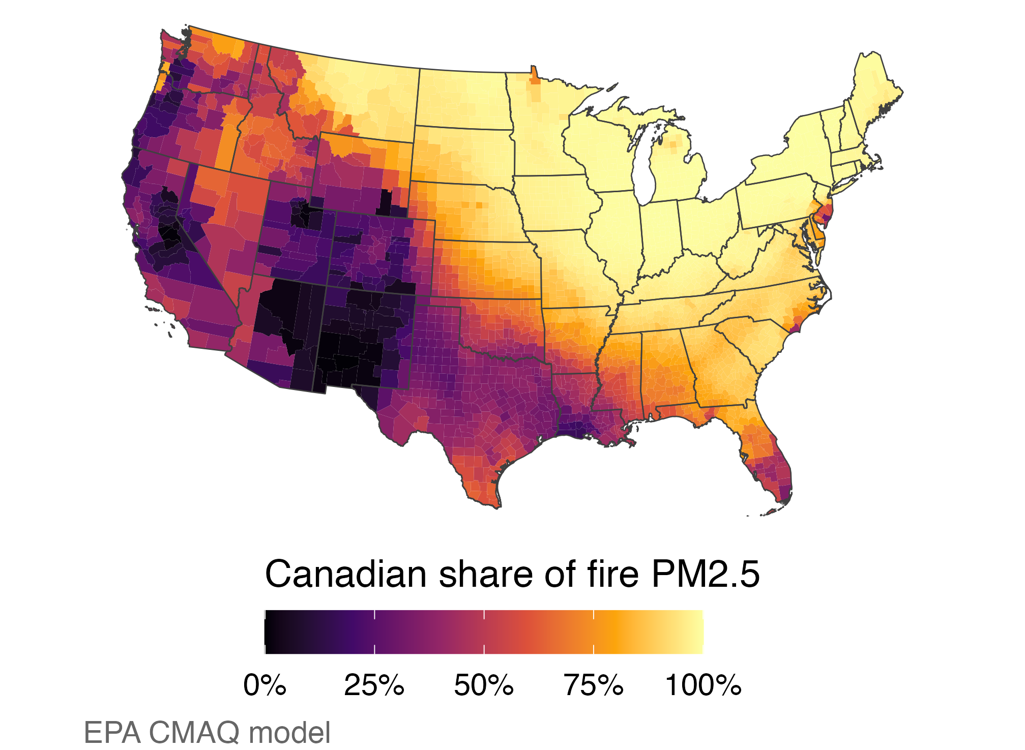
🇨🇦 Modeled share of fire smoke from Canada

ember_june <- ember |>
  group_by(GEOID) |>
  summarize(all = mean(pm25_all_fires),
    canada = mean(pm25_canada_fires)) |>
  mutate(share = canada / all)

counties |>
  left_join(ember_june, by = "GEOID") |>
  ggplot(aes(fill = share)) +
  geom_sf(color = NA) + state_lines +
  scale_fill_viridis_c(
    option = "inferno", limits = c(0, 1),
    labels = percent,
    name = "Canadian share of fire PM2.5"
  ) +
  us_albers + labs(caption = "EPA CMAQ model")

Modeled Canadian share of fire PM2.5 is high across the northern Midwest and Northeast and lower across much of the West and South.

  • Median county share: 91%. This is a model, not a measurement.

📊 Is the data really spatial?

📈 Timing is easier to read in a line chart

regional_daily <- smoke_day |>
  left_join(st_drop_geometry(counties),
            by = "GEOID") |>
  group_by(region, date) |>
  summarize(smoke = weighted.mean(
    smoke_pm25, pop_2020), .groups = "drop")

ggplot(regional_daily,
       aes(date, smoke, color = region)) +
  geom_line(linewidth = 1) +
  scale_color_manual(values = region_colors) +
  theme_minimal(base_size = 13) +
  theme(legend.position = "top") +
  labs(x = NULL, color = NULL,
       y = "Smoke PM2.5 (µg/m³)")

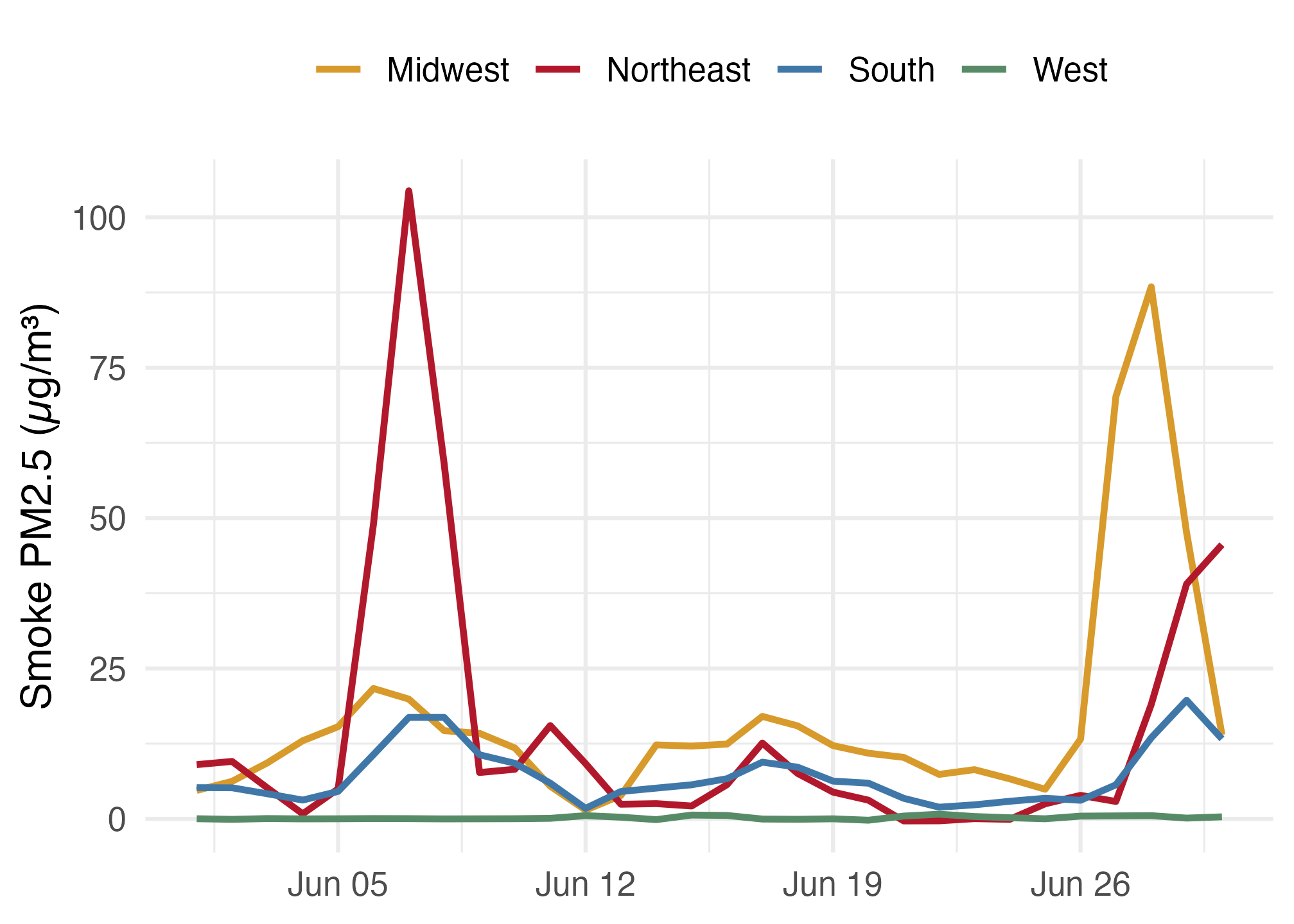
Daily June 2023 smoke PM2.5 by Census region; the Northeast spikes near June 7, the Midwest near June 28, and the West stays low.

  • Northeast peak: June 7 (104 µg/m³). Midwest peak: June 28 (88).

🗺️ Counties are containers, not the smoke itself

june7_area <- smoke_june7 |>
  # st_area() gives m² on the sphere; / 1e6 gives km²
  mutate(area_km2 = as.numeric(st_area(geometry)) / 1e6) |>
  st_drop_geometry()

june7_area |>
  summarize(
    people_weighted = weighted.mean(smoke_pm25, pop_2020),
    area_weighted   = weighted.mean(smoke_pm25, area_km2),
    simple_mean     = mean(smoke_pm25))
# A tibble: 1 × 3
  people_weighted area_weighted simple_mean
            <dbl>         <dbl>       <dbl>
1            28.9          10.3        18.0
  • Smoke is a continuous field; a county value averages a 15 km grid, weighted by population.
  • Same day, three “national averages”: say which weight you used.

✅ Wrap-up

✅ Checklist for an honest map: before you draw

  • Projection fits the area: Albers for the lower 48, Lambert for North America.
  • Keys checked: GEOID as text, boundary year matches data year, anti_join() returns zero rows.
  • Rate or count? County totals mostly map population.
  • Missing stays missing (grey); never code it as zero.

✅ Checklist for an honest map: on the page

  • Scale and bins are stated, with reasons (35 µg/m³ = EPA daily standard for total PM2.5).
  • Time convention is stated: HMS date is the UTC date; FIRMS local_date is the local solar date; smoke, EMBER, and AQS are calendar days.
  • Units, date, geography, and source are in the caption.
  • Models and plumes are labelled as what they are: modeled, or overhead.

📚 Data sources and licences

Data Source Licence
County and state boundaries, population U.S. Census Bureau, 2020 cartographic boundaries and centers of population Public domain
Province boundaries Statistics Canada, 2021 boundary files Statistics Canada Open Licence
Smoke PM2.5 (daily, monthly) CSU kriged smoke PM2.5, Pierce et al., Dryad DOI 10.5061/dryad.k0p2ngfhv CC0
Modeled fire PM2.5 EPA EMBER CMAQ runs, Zenodo 13737754 CC BY 4.0
Monitor PM2.5 EPA Air Quality System, daily PM2.5 Public domain
Smoke plumes NOAA Hazard Mapping System Public domain
Fire detections NASA FIRMS MODIS C6.1, doi:10.5067/FIRMS/MODIS/MCD14ML Open; cite NASA FIRMS
Burned-area perimeters Canadian Forest Service, CWFIS National Burned Area Composite Open Government Licence – Canada

Methods: Healy, Data Visualization, ch. 7 “Draw Maps” (socviz.co); DANL 310 Lecture 8. Build script: wildfire-maps-lecture/R/build_wildfire_map_data.R.

📌 Main takeaways

  • sf keeps geometry in one column, so dplyr verbs and joins just work.
  • Draw in a projection with coord_sf(); st_transform() changes the data, and layers must share a CRS before a join.
  • A choropleth’s message depends on keys, rates, bins, and missing values.
  • Layer points, plumes, and polygons, then ask whether a map is the best chart.

If you could add one more layer to the June 7 map to show who breathed the smoke, what would it be, and how could it still mislead?