Lecture 2

Data Transformation with dplyr

Byeong-Hak Choe

bchoe@geneseo.edu

SUNY Geneseo

August 26, 2026

🎯 Review outcome: build an auditable environmental-data pipeline

By the end of class, you should be able to:

1. choose a dplyr verb from the research question;
2. explain what one row represents before and after each step;
3. audit missingness, duplicates, and category imbalance; and
4. turn a pipeline into a defensible one-sentence finding.

Note

The goal is not to memorize verbs. It is to make each transformation serve the question.

Ask students to name one dplyr verb they use confidently and one they tend to look up. Frame the session as retrieval and transfer, not a first exposure.

🌍 Environmental questions become data pipelines

🧭 Start with the unit of observation—not the verb

Data	One row represents	What is missing from the file?
GHG inventory	One party × year × sector record	A unit label and documentation
Climate tweets	One stored tweet-text row	Sentiment, strength, ID, date, user, and place

Warning

If you cannot finish the sentence “one row represents…,” do not summarize yet.

The tweet labels can be recovered from filenames, but IDs, dates, users, and locations cannot. Distinguish a stored row from a verified unique tweet.

📥 Read the data and keep provenance visible

library(tidyverse)

ghg <- read_csv(
  "https://bcdanl.github.io/data/GHG_emissions_by.csv"
)

tweets <- bind_rows(
  positive_weak = read_csv(
    "https://bcdanl.github.io/data/UStweets_positive_weak_2017.csv"
  ),
  positive_strong = read_csv(
    "https://bcdanl.github.io/data/UStweets_positive_strong_2017.csv"
  ),
  negative_weak = read_csv(
    "https://bcdanl.github.io/data/UStweets_negative_weak_2017.csv"
  ),
  negative_strong = read_csv(
    "https://bcdanl.github.io/data/UStweets_negative_strong_2017.csv"
  ),
  .id = "sample"
)

Keep together: source URL · access date · row definition · units · known limitations.

The full tweet URLs appear in the setup chunk and later binding example. Point out that object names describe content rather than the software operation.

🧪 Audit before you answer

ghg |>
  summarise(
    rows = n(),
    parties = n_distinct(Party),
    first_year = min(Year),
    last_year = max(Year),
    sectors = n_distinct(Sector),
    missing_values =
      sum(is.na(GHG_emissions))
  )

# A tibble: 1 × 6
   rows parties first_year last_year sectors missing_values
  <int>   <int>      <dbl>     <dbl>   <int>          <int>
1  7224      43       1990      2017       6           1176

Read the output as evidence

• 7,224 rows
• 43 parties
• 1990–2017
• 6 sectors
• 1,176 missing reported values

Next question: Where are those missing values concentrated?

Have students predict the output grain: one row, because there is no group_by(). Then ask why sum(is.na()) is often more useful than merely noticing NA in a preview.

🧰 Ask what should change

Research move	What changes?	Verb
Narrow the evidence	Rows	filter()
Focus the variables	Columns	select()
Improve names or placement	Column metadata/order	rename(), relocate()
Surface high or low cases	Row order/subset	arrange(), slice_*()
Create a measure or flag	Values/columns	mutate()
Change the analytical grain	Number of rows	group_by() + summarise()
Audit repeated rows	Rows or a count	distinct(), n_distinct()

Use this as the retrieval map for the rest of class. The same data can support many pipelines; the question determines the appropriate row and column changes.

🧰 Review the core dplyr verbs

🔎 filter() narrows rows; it does not choose columns

us_focus <- ghg |>
  filter(
    Party ==
      "United States of America",
    Sector %in%
      c("Energy", "Waste"),
    Year >= 2005,
    !is.na(GHG_emissions)
  )

Four conditions, one narrower question.

Ask which conditions are categorical, temporal, and missing-data checks. Emphasize comma-separated conditions as AND.

🗂️ select(), rename(), and relocate() make the table legible

ghg_working <- ghg |>
  select(Party, Year, Sector, GHG_emissions) |>
  rename(
    party = Party,
    year = Year,
    sector = Sector,
    emissions = GHG_emissions
  ) |>
  relocate(year, party, sector)

Verb	Rule to remember
select()	Keeps or removes columns
rename()	Uses new_name = old_name
relocate()	Changes position, not values

Ask what the row count should be after this pipeline: still 7,224. Column operations do not change the unit of observation.

↕️ arrange() reveals extremes; slice_*() keeps them

ghg |>
  filter(!is.na(GHG_emissions)) |>
  select(
    Party, Year, Sector, GHG_emissions
  ) |>
  arrange(desc(GHG_emissions)) |>
  slice_head(n = 3)

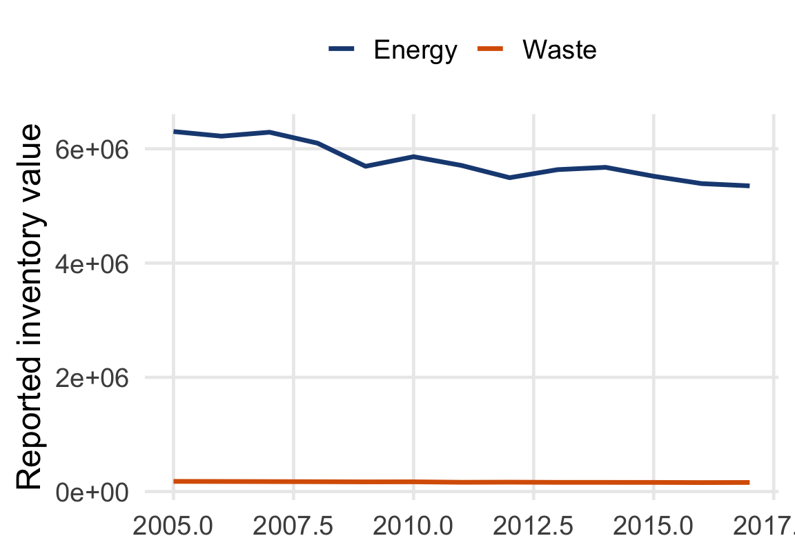
# A tibble: 3 × 4
  Party                     Year Sector GHG_emissions
  <chr>                    <dbl> <chr>          <dbl>
1 United States of America  2005 Energy      6302258.
2 United States of America  2007 Energy      6290186.
3 United States of America  2004 Energy      6285300.

Note

arrange() changes order. slice_head() changes which rows remain.

Ask whether the largest values necessarily identify the largest emitters. The file lacks a unit label and includes the EU aggregate alongside individual parties, so ranking requires interpretation.

🧮 mutate() adds variables without reducing rows

ghg_change <- ghg |>
  group_by(Party, Sector) |>
  arrange(Year, .by_group = TRUE) |>
  mutate(
    annual_change = GHG_emissions - lag(GHG_emissions),
    decreased = annual_change < 0
  ) |>
  ungroup()

Mental check: lag() only means “previous” after the rows are ordered correctly.

Ask students what happens in the first year of each group: annual_change is NA. Reinforce that grouped mutate computes within group but keeps the same number of rows.

👥 group_by() + summarise() changes the grain

ghg |>
  filter(Year == 2017) |>
  group_by(Sector) |>
  summarise(
    reporting_parties = sum(!is.na(GHG_emissions)),
    total_reported = sum(GHG_emissions, na.rm = TRUE),
    .groups = "drop"
  ) |>
  arrange(desc(total_reported))

Output grain: 6 rows—one per sector—with the number of reporting parties kept visible.

Tip

Before: one row per party × year × sector. After: one row per sector.

Separate the two missing-data decisions: count reporters, then compute a reported-value total. na.rm=TRUE does not make missing reports equal to zero.

🔁 A pipeline should read like the question

Question: How did each U.S. sector change from 1990 to 2017?

us_change <- ghg |>
  filter(Party == "United States of America",
         Year %in% c(1990, 2017)) |>
  arrange(Sector, Year) |>
  group_by(Sector) |>
  summarise(start = first(GHG_emissions),
            end = last(GHG_emissions),
            .groups = "drop") |>
  mutate(change = end - start) |>
  arrange(change)

us_change

Endpoint result: Waste = −57,125 · Energy = +25,415 · Other = missing

Ask students to narrate each line in ordinary language. Waste declines in the file; energy is roughly flat between the endpoints; Other is missing at both endpoints.

⚠️ Percent change needs a denominator check

us_change |>
  mutate(
    pct_change = if_else(
      start > 0,
      100 * change / start,
      NA_real_
    )
  )

With this rule: Waste = −26.4% · Energy = +0.5% · LULUCF and Other = NA

Warning

For U.S. LULUCF, the 1990 value is negative. A familiar percent-change formula would be difficult to interpret. For “Other,” the endpoints are missing.

This is the bridge from syntax review to research judgment. Ask why a negative baseline changes the meaning of percent change and what alternative—absolute change, separate source/sink measures, or domain-specific documentation—might be more appropriate.

🐦 Climate tweets: same verbs, messier data

🧩 File names contain data, too

tweets <- bind_rows(
  positive_weak = read_csv(
    "https://bcdanl.github.io/data/UStweets_positive_weak_2017.csv"
  ),
  positive_strong = read_csv(
    "https://bcdanl.github.io/data/UStweets_positive_strong_2017.csv"
  ),
  negative_weak = read_csv(
    "https://bcdanl.github.io/data/UStweets_negative_weak_2017.csv"
  ),
  negative_strong = read_csv(
    "https://bcdanl.github.io/data/UStweets_negative_strong_2017.csv"
  ),
  .id = "sample"
) |>
  mutate(
    sentiment = if_else(
      str_starts(sample, "positive"), "positive", "negative"
    ),
    strength = if_else(
      str_ends(sample, "strong"), "strong", "weak"
    )
  )

Result: 167,050 rows × 4 columns.

The supplied CSVs contain only content. The .id argument preserves which source file each row came from; mutate then recovers the two labels encoded in the filenames.

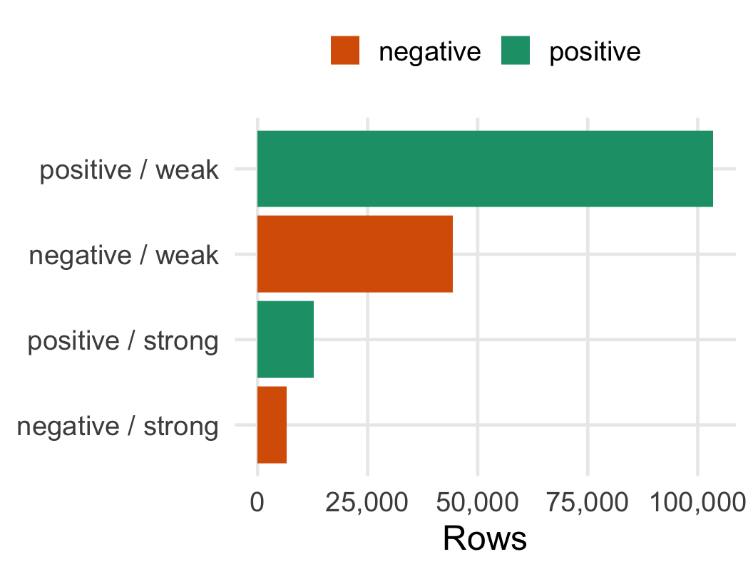
📊 Count first: the four samples are not balanced

counts <- tweets |>
  count(
    sentiment, strength,
    name = "tweets"
  ) |>
  mutate(
    share = tweets / sum(tweets)
  ) |>
  arrange(desc(tweets))

61.96% of rows are positive/weak; only 3.92% are negative/strong.

Ask why an overall percentage or model accuracy could be misleading when groups have different sizes. count() is group_by() plus summarise(n = n()) in one step.

🧯 A file can parse cleanly and still contain dirty text

tweets |>
  mutate(suspicious_encoding = str_detect(content, "[âÂ]")) |>
  summarise(
    rows = n(),
    flagged = sum(suspicious_encoding),
    flagged_share = mean(suspicious_encoding)
  )

• read_csv() reports no parsing problems.
• The simple screen flags 130,347 rows (78.0%).
• Strings such as … and Â suggest mojibake.

Warning

This is an audit flag—not a safe replacement rule. Repair requires knowing the original encoding history.

Distinguish syntactically valid CSV from semantically clean text. Avoid promising that a global replacement fixes the data.

🌪️ Build a topic comparison from three verbs

Question: Which labeled samples contain tweets mentioning hurricanes?

hurricane_pattern <- regex(
  "\\bhurricanes?\\b",
  ignore_case = TRUE
)

tweets |>
  filter(str_detect(content, hurricane_pattern)) |>
  count(sentiment, strength,
        name = "tweets") |>
  mutate(share = tweets / sum(tweets)) |>
  arrange(desc(tweets))

3,069 matches: Positive/weak 1,824 · Negative/weak 970 · Negative/strong 151 · Positive/strong 124

The result describes the labeled sample, not public opinion or all U.S. tweets. Ask students to state that limitation before interpreting the shares.

🧬 across() repeats the same summary safely

tweets |>
  mutate(
    hurricane = str_detect(content,
      regex("\\bhurricanes?\\b", ignore_case = TRUE)),
    wildfire = str_detect(content,
      regex("\\bwildfires?\\b", ignore_case = TRUE)),
    flood = str_detect(content,
      regex("\\bflood(s|ed|ing)?\\b", ignore_case = TRUE)),
    drought = str_detect(content,
      regex("\\bdroughts?\\b", ignore_case = TRUE))
  ) |>
  summarise(
    across(hurricane:drought, \(x) sum(x, na.rm = TRUE))
  )

Tweet-row flags: hurricanes 3,069 · wildfires 1,282 · floods 2,409 · droughts 1,080

These are tweet-row flags, not word frequencies. A row can contribute to more than one topic count. across() is useful when the same operation genuinely applies to several columns.

🧹 Duplicate handling changes the research quantity

tweets |>
  group_by(sentiment, strength) |>
  summarise(
    rows = n(),
    unique_text = n_distinct(content),
    duplicate_rows = rows - unique_text,
    duplicate_share = duplicate_rows / rows,
    .groups = "drop"
  ) |>
  arrange(desc(duplicate_share))

Audit: 7,108 repeated rows · weak groups ≈ 4.6% · strong groups = 1.5%–2.8%

Note

Use distinct(content, .keep_all = TRUE) only when the unit should be unique text. Repeats may be behavior, not error.

There is no tweet ID, so exact text is the only available key and may collapse distinct events. Ask what substantive quantity changes when duplicates are removed.

🛠️ Practice and handoff

🧠 Choose the verb from the question

1. Keep only 2017 Waste records.
2. Add annual change within each party and sector.
3. Return one row per sector with a median.
4. Keep the three largest values within each sector.
5. Count unique tweet texts by sentiment and strength.

1. filter()
2. grouped mutate() + lag()
3. group_by() + summarise()
4. grouped slice_max()
5. n_distinct() inside summarise()

Give students 60–90 seconds before revealing the right column. Ask them to predict the output grain for each task.

✅ A defensible pipeline leaves an audit trail

Before interpreting a result, confirm:

• Unit: What does one output row represent?
• Scope: Which rows and columns remain?
• Order: Did any lag, first, last, or slice depend on sorting?
• Missingness: What did NA mean, and how was it handled?
• Duplicates: Are repeated rows error, exposure, or behavior?
• Claim: What can this sample support—and what can it not?

Classwork: Build and audit a greenhouse-gas change pipeline →

Close by linking the syntax review to each student’s Question + Data Scan. The next step is to apply this audit trail to their own candidate source.