import numpy as np
import pandas as pd
import matplotlib.pyplot as plt
import seaborn as sns

from sklearn.preprocessing import scale # zero mean & one s.d.
from sklearn.linear_model import LassoCV, lasso_path
from sklearn.model_selection import train_test_split
from sklearn.metrics import mean_squared_errorHomework 4 - Part 1: Lasso Linear Regerssion - Model 3 with Discussions
Beer Markets with Big Demographic Design
#beer = pd.read_csv("https://bcdanl.github.io/data/beer_markets_xbeer_xdemog.zip")
#beer = pd.read_csv("https://bcdanl.github.io/data/beer_markets_xbeer_brand_xdemog.zip")
beer = pd.read_csv("https://bcdanl.github.io/data/beer_markets_xbeer_brand_promo_xdemog.zip")
X = beer.drop('ylogprice', axis = 1)
y = beer['ylogprice']X_train, X_test, y_train, y_test = train_test_split(X, y, test_size=0.2, random_state=42)
y_train = y_train.values
y_test = y_test.values# LassoCV with a range of alpha values
lasso_cv = LassoCV(n_alphas = 100,
alphas = None, # alphas=None automatically generate 100 candidate alpha values
cv = 5,
random_state=42,
max_iter=100000)lasso_cv.fit(X_train.values, y_train)
#lasso_cv.fit(X_train.values, y_train.ravel())
print("LassoCV - Best alpha:", lasso_cv.alpha_)LassoCV - Best alpha: 0.00022539867869301466# Create a DataFrame including the intercept and the coefficients:
coef_lasso_beer = pd.DataFrame({
'predictor': list(X_train.columns),
'coefficient': list(lasso_cv.coef_),
'exp_coefficient': np.exp( list(lasso_cv.coef_) )
})
# Evaluate
y_pred_lasso = lasso_cv.predict(X_test)
mse_lasso = mean_squared_error(y_test, y_pred_lasso)
print("LassoCV - MSE:", mse_lasso)LassoCV - MSE: 0.02863537005154527coef_lasso_beer_n0 = coef_lasso_beer[coef_lasso_beer['coefficient'] != 0]X_train.shape[1]2655coef_lasso_beer_n0.shape[0]163coef_lasso_beer_n0| predictor | coefficient | exp_coefficient | |
|---|---|---|---|
| 0 | logquantity | -0.136277 | 0.872601 |
| 1 | container_CAN | -0.056243 | 0.945309 |
| 2 | brandBUSCH_LIGHT | -0.072086 | 0.930451 |
| 4 | brandMILLER_LITE | 0.001853 | 1.001854 |
| 5 | brandNATURAL_LIGHT | -0.457505 | 0.632861 |
| ... | ... | ... | ... |
| 2372 | marketRURAL_WEST_VIRGINIA:npeople2 | -0.032313 | 0.968203 |
| 2385 | marketTAMPA:npeople2 | 0.018947 | 1.019127 |
| 2386 | marketURBAN_NY:npeople2 | 0.001501 | 1.001502 |
| 2426 | marketRALEIGH-DURHAM:npeople3 | -0.005387 | 0.994627 |
| 2582 | marketEXURBAN_NJ:npeople5plus | 0.080731 | 1.084079 |
163 rows × 3 columns
# Compute the mean and standard deviation of the CV errors for each alpha.
mean_cv_errors = np.mean(lasso_cv.mse_path_, axis=1)
std_cv_errors = np.std(lasso_cv.mse_path_, axis=1)

plt.figure(figsize=(8, 6))
plt.errorbar(lasso_cv.alphas_, mean_cv_errors, yerr=std_cv_errors, marker='o', linestyle='-', capsize=5)
plt.xscale('log')
plt.xlabel('Alpha')
plt.ylabel('Mean CV Error (MSE)')
plt.title('Cross-Validation Error vs. Alpha')
#plt.gca().invert_xaxis()  # Optionally invert the x-axis so lower alphas (less regularization) appear to the right.
plt.axvline(x=lasso_cv.alpha_, color='red', linestyle='--', label='Best alpha')
plt.legend()
plt.show()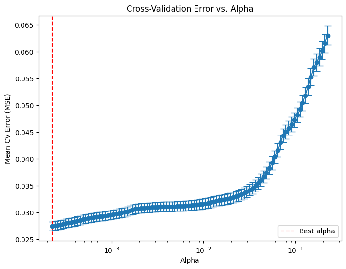
# Compute the coefficient path over the alpha grid that LassoCV used
alphas, coefs, _ = lasso_path(X_train, y_train,
                              alphas=lasso_cv.alphas_,
                              max_iter=100000)

# Count nonzero coefficients for each alpha (coefs shape: (n_features, n_alphas))
nonzero_counts = np.sum(coefs != 0, axis=0)

# Plot the number of nonzero coefficients versus alpha
plt.figure(figsize=(8,6))
plt.plot(alphas, nonzero_counts, marker='o', linestyle='-')
plt.xscale('log')
plt.xlabel('Alpha')
plt.ylabel('Number of nonzero coefficients')
plt.title('Nonzero Coefficients vs. Alpha')
#plt.gca().invert_xaxis()  # Lower alphas (less regularization) on the right
plt.axvline(x=lasso_cv.alpha_, color='red', linestyle='--', label='Best alpha')
plt.legend()
plt.show()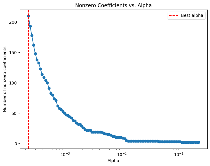
# Compute the lasso path. Note: we use np.log(y_train) because that's what you used in LassoCV.
alphas, coefs, _ = lasso_path(X_train, y_train,
                              alphas=lasso_cv.alphas_,
                              max_iter=100000)
plt.figure(figsize=(8, 6))
# Iterate over each predictor and plot its coefficient path.
for i, col in enumerate(X_train.columns):
    plt.plot(alphas, coefs[i, :], label=col)

plt.xscale('log')
plt.xlabel('Alpha')
plt.ylabel('Coefficient value')
plt.title('Lasso Coefficient Paths')
#plt.gca().invert_xaxis()  # Lower alphas (weaker regularization) to the right.
#plt.legend(bbox_to_anchor=(1.05, 1), loc='upper left')
plt.axvline(x=lasso_cv.alpha_, color='red', linestyle='--', label='Best alpha')
#plt.legend()
plt.show()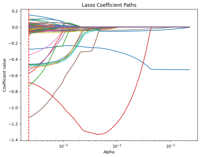
Best Alphas
Model 1: 0.000082
Model 2: 0.000225
Model 3: 0.000225
Sensitivity Estimates without Demographic Controls (Homework 2)
| Model 1 | Model 2 | Model 3 (no Promo) | Model 3 (with Promo) | |
|---|---|---|---|---|
| BUD | -0.142 | -0.146 | -0.140 | -0.148 = −0.140 − 0.008 |
| BUSCH | -0.142 | -0.159 = −0.146 − 0.013 |
-0.161 = −0.140 − 0.021 |
-0.122 = −0.140 − 0.021 − 0.008 + 0.047 |
| COORS | -0.142 | -0.146 = −0.146 − 0 |
-0.148 = −0.140 − 0.008 |
-0.119 = −0.140 − 0.008 − 0.008 + 0.037 |
| MILLER | -0.142 | -0.163 = −0.146 − 0.017 |
-0.163 = −0.140 − 0.023 |
-0.119 = −0.140 − 0.023 − 0.008 + 0.052 |
| NATURAL | -0.142 | -0.094 = −0.146 + 0.052 |
-0.103 = −0.140 + 0.037 |
-0.040 = −0.140 + 0.037 − 0.008 + 0.071 |
Sensitivity Estimates with Demographic Controls
| Model 1 | Model 2 | Model 3 (no Promo) | Model 3 (with Promo) | |
|---|---|---|---|---|
| BUD | -0.1429 | -0.1408 | -0.1363 | -0.1403 = −0.1363 + 0.0040 |
| BUSCH | -0.1429 | -0.1719 = −0.1408 − 0.0311 |
-0.1708 = −0.1363 − 0.0345 |
-0.1418 = −0.1363 − 0.0345 + 0.0040 + 0.025 |
| COORS | -0.1429 | -0.1414 = −0.1408 − 0.0006 |
-0.1365 = −0.1363 − 0.0002 |
-0.1355 = −0.1363 − 0.0002 + 0.0040 - 0.0030 |
| MILLER | -0.1429 | -0.1443 = −0.1408 − 0.0035 |
-0.1401 = −0.1363 − 0.0038 |
-0.1353 = −0.1363 − 0.0038 + 0.0040 + 0.0008 |
| NATURAL | -0.1429 | -0.1113 = −0.1408 + 0.0295 |
-0.1105 = −0.1363 + 0.0258 |
-0.1058 = −0.1363 + 0.0258 + 0.0040 + 0.0007 |
Sensitivity Visuals with & without Demographic Controls
# Slopes (inverse elasticities)
model1_slope = -0.142
model2_slopes = {
    'Bud': -0.146,
    'Busch': -0.159,
    'Coors': -0.146,
    'Miller': -0.163,
    'Natural': -0.094
}
model3_full_slopes = {
    'Bud': -0.140,
    'Busch': -0.161,
    'Coors': -0.148,
    'Miller': -0.163,
    'Natural': -0.103
}
model3_promo_slopes = {
    'Bud': -0.148,
    'Busch': -0.122,
    'Coors': -0.119,
    'Miller': -0.096,
    'Natural': -0.077
}

model1_demog_slope = -0.1429
model2_demog_slopes = {
    'Bud': -0.1408,
    'Busch': -0.1719,
    'Coors': -0.1414,
    'Miller': -0.1443,
    'Natural': -0.1113
}
model3_demog_full_slopes = {
    'Bud': -0.1363,
    'Busch': -0.1708,
    'Coors': -0.1365,
    'Miller': -0.1401,
    'Natural': -0.1105
}
model3_demog_promo_slopes = {
    'Bud': -0.1403,
    'Busch': -0.1418,
    'Coors': -0.1355,
    'Miller': -0.1353,
    'Natural': -0.1058
}

# Create range of log(sales) values
x = np.linspace(0, 10, 100)

# Set up a 2x4 grid of subplots
fig, axes = plt.subplots(2, 4, figsize=(16, 8), sharex=True, sharey=True)

# First row: models without demographics
# Model 1
ax = axes[0, 0]
ax.plot(x, model1_slope * x, color='tab:blue', label='All Brands')
ax.set_title('Model 1')
ax.set_ylabel('log(price)')
ax.grid(True)
ax.legend(loc='lower left')

# Model 2
ax = axes[0, 1]
for brand, slope in model2_slopes.items():
    ax.plot(x, slope * x, label=brand)
ax.set_title('Model 2')
ax.grid(True)
ax.legend(loc='lower left')

# Model 3 Full (No Promo)
ax = axes[0, 2]
for brand, slope in model3_full_slopes.items():
    ax.plot(x, slope * x, label=brand)
ax.set_title('Model 3 Full')
ax.grid(True)
ax.legend(loc='lower left')

# Model 3 Promo
ax = axes[0, 3]
for brand, slope in model3_promo_slopes.items():
    ax.plot(x, slope * x, label=brand)
ax.set_title('Model 3 Promo')
ax.grid(True)
ax.legend(loc='lower left')

# Second row: models with demographics
# Model 1 + Demog
ax = axes[1, 0]
ax.plot(x, model1_demog_slope * x, color='tab:orange', label='All Brands + Demog')
ax.set_title('Model 1 (+ Demog)')
ax.set_ylabel('log(price)')
ax.set_xlabel('log(sales)')
ax.grid(True)
ax.legend(loc='lower left')

# Model 2 + Demog
ax = axes[1, 1]
for brand, slope in model2_demog_slopes.items():
    ax.plot(x, slope * x, label=brand)
ax.set_title('Model 2 (+ Demog)')
ax.set_xlabel('log(sales)')
ax.grid(True)
ax.legend(loc='lower left')

# Model 3 Full + Demog
ax = axes[1, 2]
for brand, slope in model3_demog_full_slopes.items():
    ax.plot(x, slope * x, label=brand)
ax.set_title('Model 3 Full (+ Demog)')
ax.set_xlabel('log(sales)')
ax.grid(True)
ax.legend(loc='lower left')

# Model 3 Promo + Demog
ax = axes[1, 3]
for brand, slope in model3_demog_promo_slopes.items():
    ax.plot(x, slope * x, label=brand)
ax.set_title('Model 3 Promo (+ Demog)')
ax.set_xlabel('log(sales)')
ax.grid(True)
ax.legend(loc='lower left')

plt.tight_layout()
plt.show()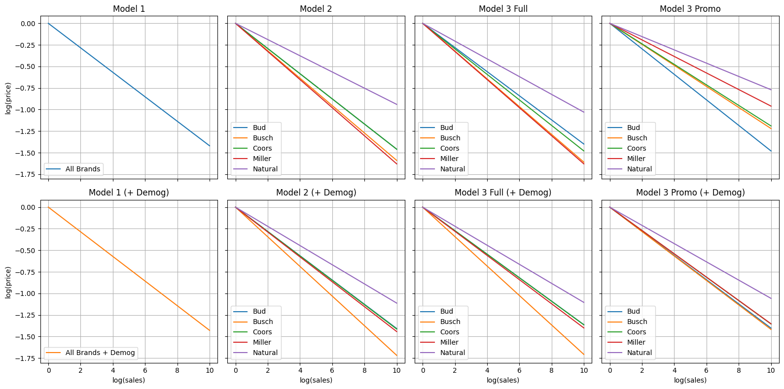
How Demographic Controls Affect Price–Volume Sensitivity
Adding demographic covariates shifts the implied own‑price elasticities by varying amounts across models and brands.
Model 1 (Common Elasticity)
| Specification | Elasticity |
|---|---|
| Without demographics | –0.1420 |
| With demographics | –0.1429 |
| Δ | –0.0009 |
| Effect | Slightly more elastic (negligible change) |
Model 2 (Brand‑Specific Elasticities)
| Brand | Without Demog | With Demog | Δ | Effect |
|---|---|---|---|---|
| Bud | –0.1460 | –0.1408 | +0.0052 | Less elastic |
| Busch | –0.1590 | –0.1719 | –0.0129 | More elastic |
| Coors | –0.1460 | –0.1414 | +0.0046 | Less elastic |
| Miller | –0.1630 | –0.1443 | +0.0187 | Much less elastic |
| Natural | –0.0940 | –0.1113 | –0.0173 | More elastic |
Interpretation: Demographics slightly dampen sensitivity for Bud, Coors, and Miller but increase it for Busch and Natural.
Model 3 Full‑Price (No Promo)
| Brand | Without Demog | With Demog | Δ | Effect |
|---|---|---|---|---|
| Bud | –0.1400 | –0.1363 | +0.0037 | Less elastic |
| Busch | –0.1610 | –0.1708 | –0.0098 | More elastic |
| Coors | –0.1480 | –0.1365 | +0.0115 | Less elastic |
| Miller | –0.1630 | –0.1401 | +0.0229 | Much less elastic |
| Natural | –0.1030 | –0.1105 | –0.0075 | More elastic |
Interpretation: Similar pattern to Model 2; demographic controls modestly increase or decrease brand‑specific slopes.
Model 3 Promotional‑Price
| Brand | Without Demog | With Demog | Δ | Effect |
|---|---|---|---|---|
| Bud | –0.1480 | –0.1403 | +0.0077 | Less elastic |
| Busch | –0.1220 | –0.1418 | –0.0198 | More elastic |
| Coors | –0.1190 | –0.1355 | –0.0165 | More elastic |
| Miller | –0.0960 | –0.1353 | –0.0393 | Much more elastic |
| Natural | –0.0770 | –0.1058 | –0.0288 | More elastic |
Interpretation: Demographic adjustments have the largest impact here, especially increasing sensitivity for Miller and others.
Summary
- Model 1: Virtually no change when demographics are added.
- Models 2 & 3 without Promo: Elasticities shift modestly by brand—some become slightly more price‑sensitive, others slightly less.
- Model 3 Promo: Most brands become notably more elastic once demographics are included. This implies that consumer characteristics play a key role in how promotions affect beer pricing.
Test Set RMSE Comparison
| Model | RMSE (no demogs) | RMSE (with demogs) |
|---|---|---|
| 1 | 0.167 | 0.0278 |
| 2 | 0.166 | 0.0290 |
| 3 | 0.165 | 0.0286 |
Including demographic controls dramatically lowers the prediction error for all three models, implying that adding demogs substantially improves prediction performance.