Homework 4 - Part 2: Tree-based Models

MLB Batting

Author

Byeong-Hak Choe

Published

April 19, 2025

Modified

May 3, 2025

import pandas as pd
import numpy as np
import seaborn as sns
import matplotlib.pyplot as plt

from sklearn.model_selection import train_test_split, KFold, cross_val_score
from sklearn.metrics import mean_squared_error

from sklearn.tree import DecisionTreeClassifier, DecisionTreeRegressor, plot_tree
from sklearn.ensemble import RandomForestRegressor

mlb_battings_2024 = pd.read_csv("https://bcdanl.github.io/data/mlb_battings_2024.csv")
mlb_battings_2024.shape

(230, 19)

mlb_battings_2024

	g	pa	hr	r	rbi	sb	bb_percent	k_percent	iso	babip	avg	obp	slg	w_oba	w_rc	bs_r	off	def	war
0	421	1858	157	334	350	29	17.9	25.6	0.370	0.341	0.304	0.433	0.674	0.455	202	-1.8	216.3	-16.4	27.0
1	473	2082	90	313	296	76	8.7	19.1	0.207	0.291	0.266	0.340	0.473	0.350	128	8.9	77.5	43.1	19.6
2	451	1996	132	326	320	90	12.2	23.3	0.309	0.332	0.296	0.385	0.605	0.411	168	10.6	169.9	-48.1	19.2
3	467	2076	72	329	291	45	11.3	15.6	0.206	0.347	0.314	0.399	0.520	0.391	153	4.7	136.8	-25.2	18.6
4	469	2035	82	304	285	110	6.2	17.8	0.217	0.316	0.288	0.336	0.505	0.356	128	19.3	84.4	28.9	18.5
...	...	...	...	...	...	...	...	...	...	...	...	...	...	...	...	...	...	...	...
225	412	1587	51	166	162	12	10.3	26.1	0.177	0.272	0.221	0.303	0.397	0.305	91	-2.2	-18.0	-41.9	-0.8
226	417	1603	53	159	189	13	5.5	25.1	0.158	0.300	0.247	0.289	0.405	0.300	87	-5.6	-30.8	-33.2	-1.0
227	288	1017	25	119	85	15	8.3	20.7	0.120	0.263	0.223	0.293	0.343	0.282	73	-1.3	-33.5	-18.2	-1.8
228	313	1105	36	124	133	15	6.1	24.2	0.160	0.261	0.221	0.268	0.381	0.280	75	-0.2	-32.8	-24.0	-2.1
229	381	1255	35	93	141	3	7.8	20.6	0.140	0.262	0.227	0.291	0.368	0.288	84	-5.1	-28.4	-34.7	-2.2

230 rows × 19 columns

Regression Tree

# Set a random seed for reproducibility
np.random.seed(42120532)
train, test = train_test_split(mlb_battings_2024, test_size=0.20, random_state=42120532)

X_train = train.drop(columns=["war"])
y_train = train["war"]

X_test = test.drop(columns=["war"])
y_test = test["war"]

# In scikit-learn, we can use min_impurity_decrease=0.005 for a similar effect.
tree_model = DecisionTreeRegressor(min_impurity_decrease=0.005, random_state=42)
# Fit the model using all predictors (all columns except 'medv')
tree_model.fit(X_train, y_train)


# Predict on training and test sets
y_train_pred = tree_model.predict(X_train)
y_test_pred = tree_model.predict(X_test)

# Calculate MSE
mse_train = mean_squared_error(y_train, y_train_pred)
mse_test = mean_squared_error(y_test, y_test_pred)

# Print the results
print(f"Training MSE: {mse_train:.3f}")
print(f"Test MSE: {mse_test:.3f}")

# Plot the initial regression tree
plt.figure(figsize=(12, 8), dpi = 300)
plot_tree(tree_model, feature_names=X_train.columns, filled=True, rounded=True)
plt.title("Regression Tree for war (Initial Fit)")
plt.show()

Training MSE: 0.092
Test MSE: 6.154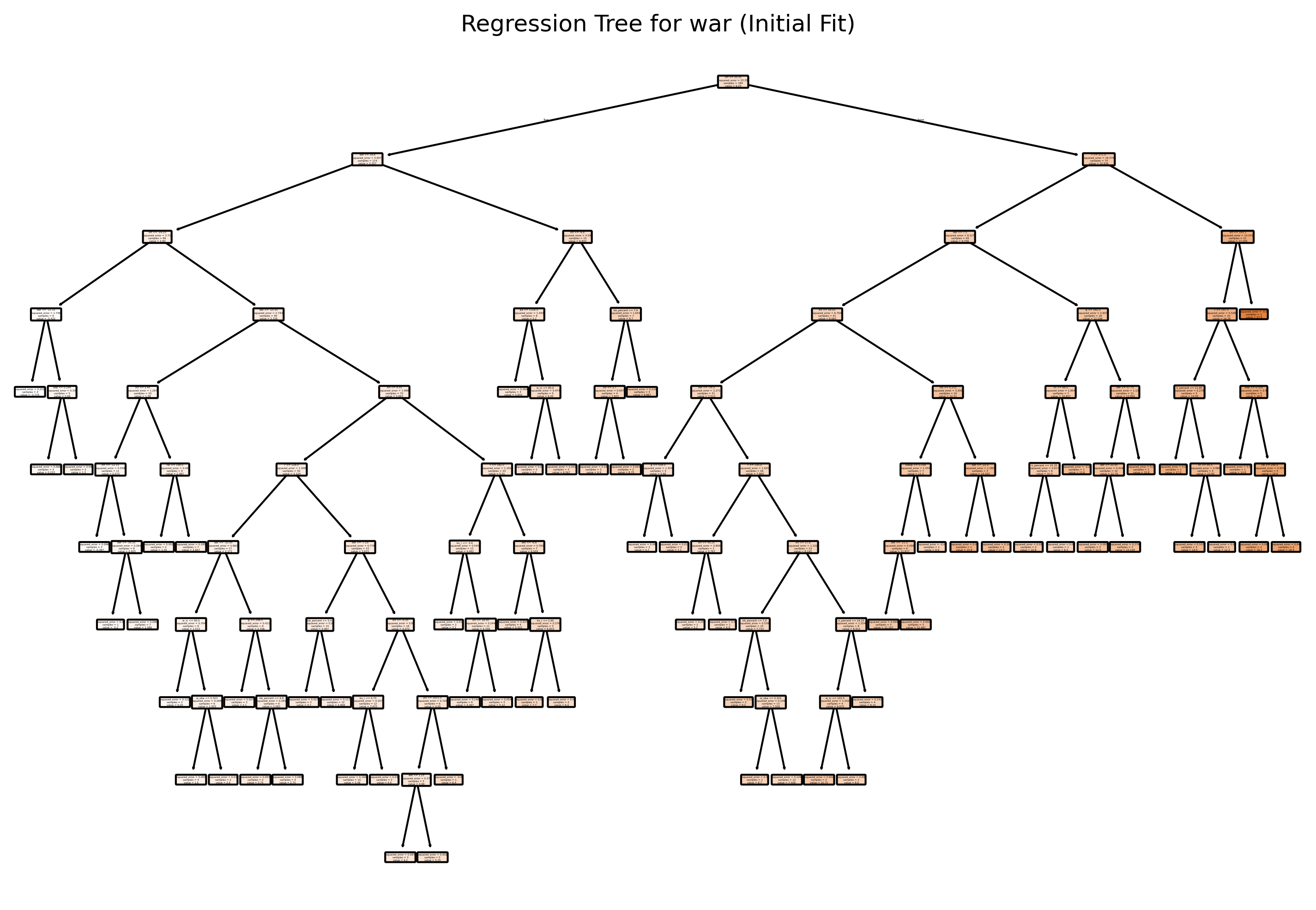

# In scikit-learn, we can use min_impurity_decrease=0.005 for a similar effect.
tree_model = DecisionTreeRegressor(max_depth=3, min_impurity_decrease=0.005, random_state=42)
# Fit the model using all predictors (all columns except 'medv')
tree_model.fit(X_train, y_train)

# Predict on training and test sets
y_train_pred = tree_model.predict(X_train)
y_test_pred = tree_model.predict(X_test)

# Calculate MSE
mse_train = mean_squared_error(y_train, y_train_pred)
mse_test = mean_squared_error(y_test, y_test_pred)

# Print the results
print(f"Training MSE: {mse_train:.3f}")
print(f"Test MSE: {mse_test:.3f}")

# Plot the initial regression tree
plt.figure(figsize=(12, 8), dpi = 300)
plot_tree(tree_model, feature_names=X_train.columns, filled=True, rounded=True)
plt.title("Regression Tree for war (Initial Fit)")
plt.show()

Training MSE: 3.61641995
Test MSE: 7.20819639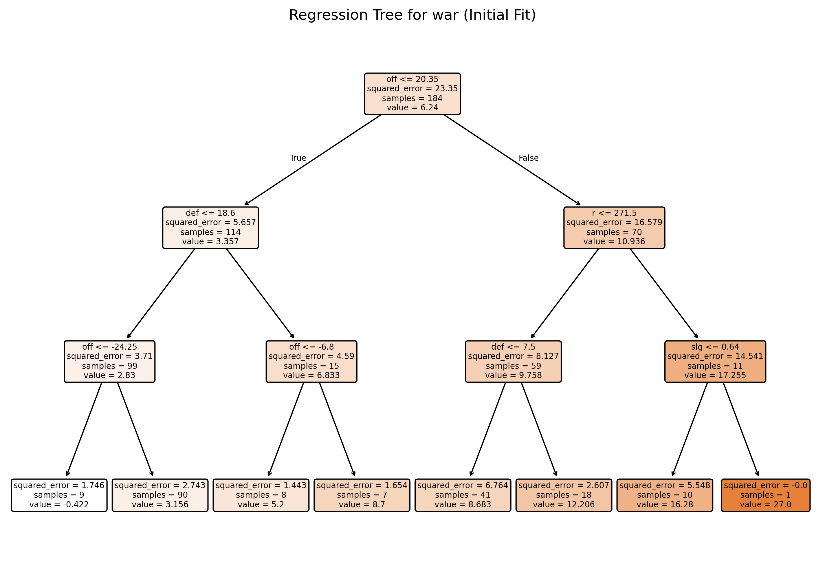

Prunning

# Obtain the cost-complexity pruning path from the initial tree
path = tree_model.cost_complexity_pruning_path(X_train, y_train)  # Get candidate ccp_alpha values and corresponding impurities
ccp_alphas = path.ccp_alphas  # Candidate pruning parameters (alpha values)
impurities = path.impurities  # Impurity values at each candidate alpha

# Exclude the maximum alpha value to avoid the trivial tree (a tree with only the root)
ccp_alphas = ccp_alphas[:-1]  # Remove the last alpha value which would prune the tree to a single node

# Set up 10-fold cross-validation
kf = KFold(n_splits=10, shuffle=True, random_state=42)  # Initialize 10-fold CV with shuffling and fixed random state
cv_scores = []  # List to store mean cross-validated scores (negative MSE)
leaf_nodes = []  # List to record the number of leaves for each pruned tree
sse = []         # List to record the sum of squared errors (SSE) on the training set

# Loop over each candidate alpha value to evaluate its performance
for ccp_alpha in ccp_alphas:
    # Create a DecisionTreeRegressor with the current ccp_alpha and other specified parameters
    clf = DecisionTreeRegressor(random_state=42,
                                ccp_alpha=ccp_alpha,
                                min_impurity_decrease=0.005)

    # Perform 10-fold cross-validation and compute negative mean squared error (MSE)
    scores = cross_val_score(clf, X_train, y_train,
                             cv=kf, scoring="neg_mean_squared_error")
    cv_scores.append(np.mean(scores))  # Append the mean CV score for the current alpha

    # Fit the tree on the training data to record additional metrics
    clf.fit(X_train, y_train)
    leaf_nodes.append(clf.get_n_leaves())  # Record the number of leaf nodes in the tree

    # Compute SSE (sum of squared errors) on the training set
    preds = clf.predict(X_train)  # Predict target values on training data
    sse.append(np.sum((y_train - preds) ** 2))  # Calculate and record SSE for training set


# Select the best alpha based on the highest (least negative) mean CV score
best_alpha = ccp_alphas[np.argmax(cv_scores)]  # Identify the alpha with the best CV performance
print("Best alpha:", best_alpha)  # Print the best alpha value

# Train the final pruned tree using the best alpha found
final_tree = DecisionTreeRegressor(random_state=42,
                                   ccp_alpha=best_alpha,
                                   min_impurity_decrease=0.005)
final_tree.fit(X_train, y_train)  # Fit the final model on the training data

len(ccp_alphas)

preds_train = final_tree.predict(train.drop(columns=["war"]))
mse_train = mean_squared_error(y_train, preds_train)
print("Train MSE:", mse_train)

preds = final_tree.predict(test.drop(columns=["war"]))
mse = mean_squared_error(y_test, preds)
print("Test MSE:", mse)

# Plot the pruned tree.
plt.figure(figsize=(16, 12), dpi=300)
plot_tree(final_tree, feature_names=X_train.columns, filled=True, rounded=True)
plt.title("Pruned Regression Tree for medv")
plt.show()

# Summary of the final tree
print("Number of leaves in the pruned tree:", final_tree.get_n_leaves())
print("Tree depth:", final_tree.get_depth())

Best alpha: 0.012181159420289953
Train MSE: 0.21034767647811128
Test MSE: 5.97171015229301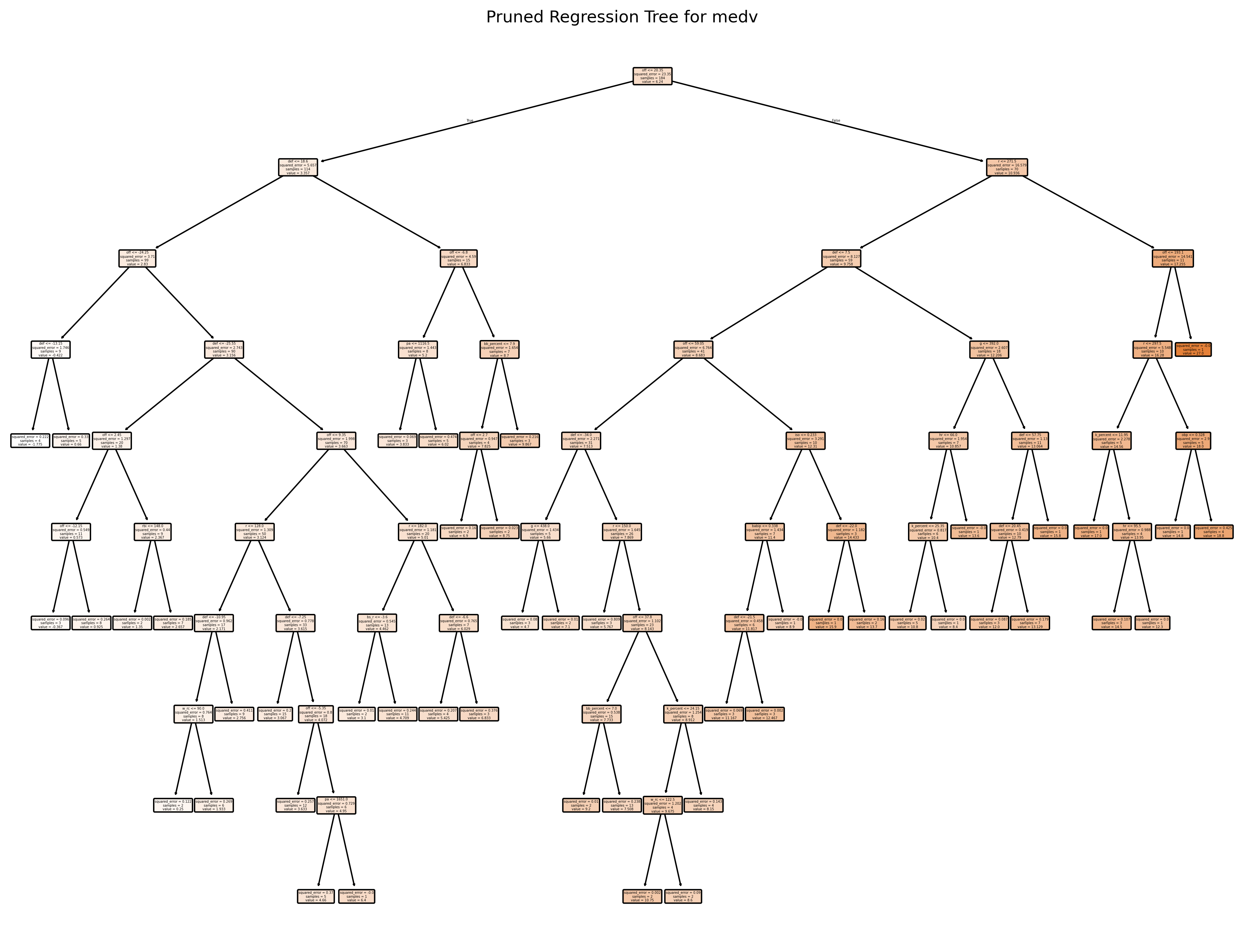

Number of leaves in the pruned tree: 47
Tree depth: 9

# Plot the average cross-validated MSE against the number of leaf nodes
negative_cv_scores = -np.array(cv_scores)

plt.figure(figsize=(8, 6), dpi=150)
plt.plot(leaf_nodes, negative_cv_scores, marker='o', linestyle='-')
plt.axvline(x=final_tree.get_n_leaves(), color='red', linestyle='--', label='Leaf Nodes = 21')  # Add vertical line at 21 leaf nodes
plt.xlabel("Number of Leaf Nodes")
plt.ylabel("Mean CV MSE")
plt.title("CV Error vs. Number of Leaf Nodes")
plt.grid(True)
plt.show()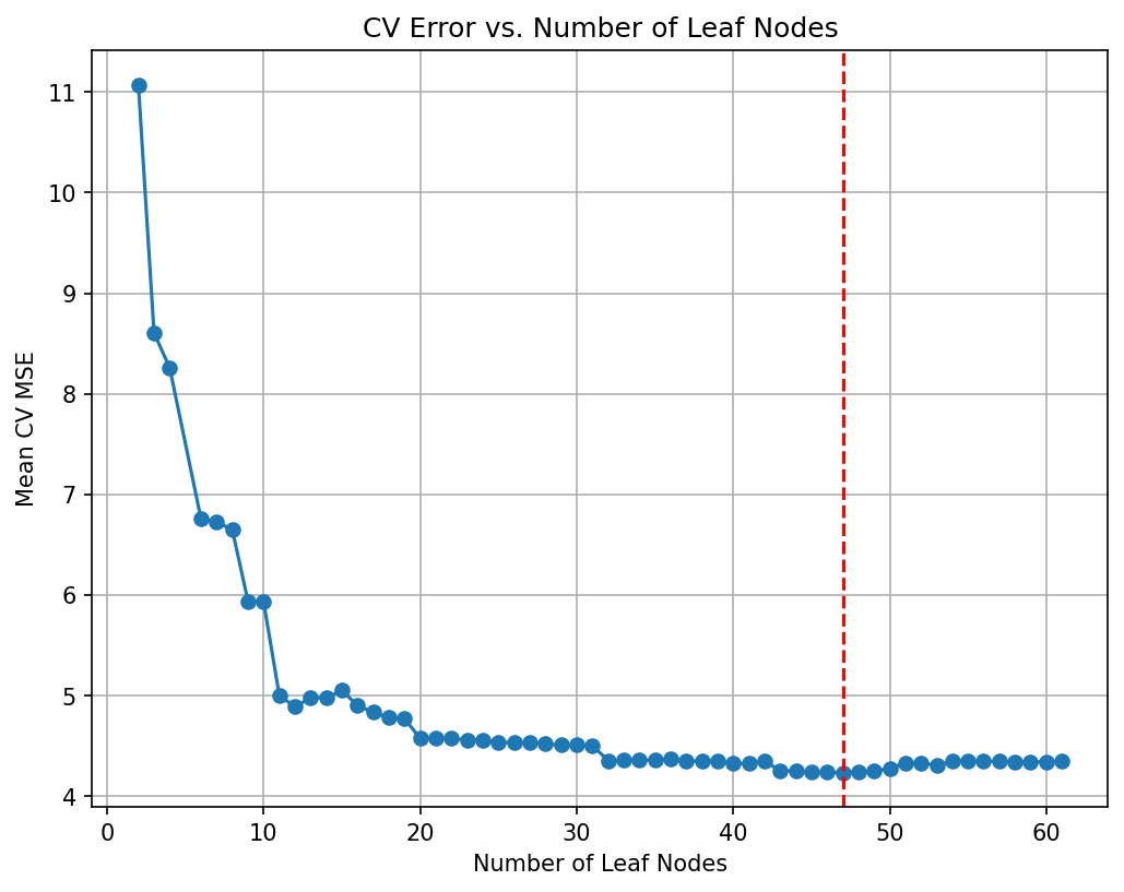

# Plot the SSE on the training against the number of leaf nodes
plt.figure(figsize=(8, 6), dpi=150)
plt.plot(leaf_nodes, sse, marker='o', linestyle='-')
plt.xlabel("Number of Leaf Nodes")
plt.ylabel("SSE")
plt.title("SSE vs. Number of Leaf Nodes")
plt.grid(True)
plt.show()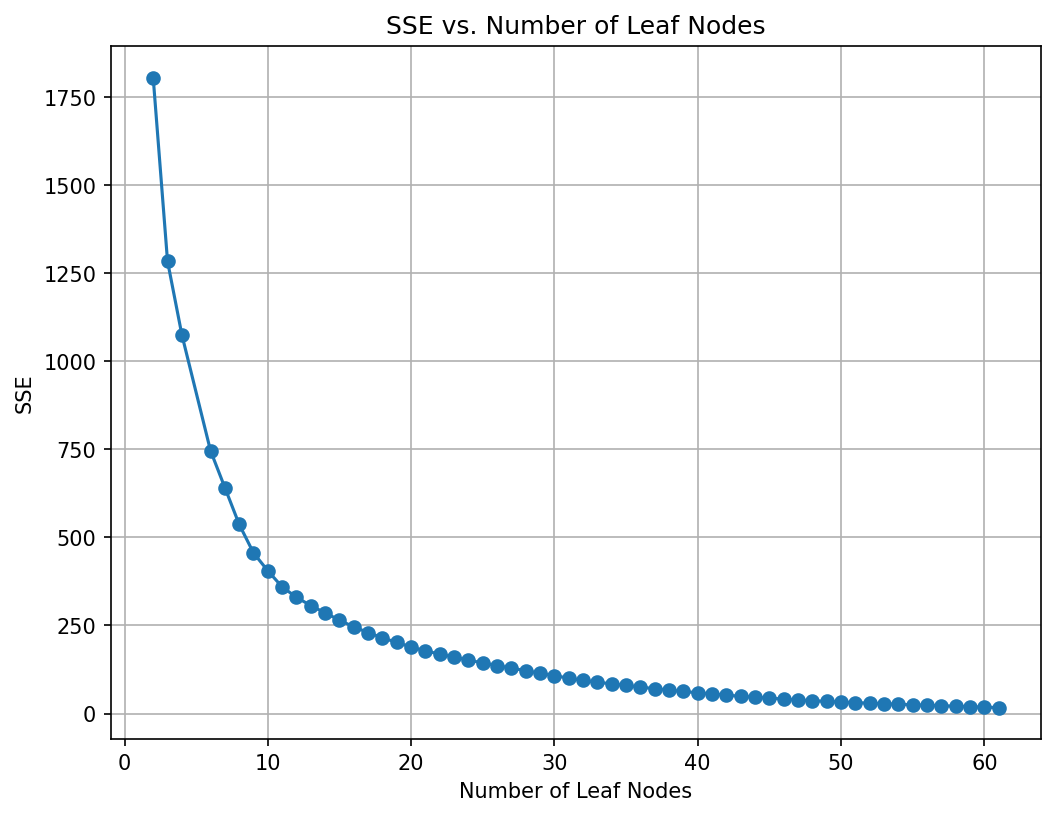

Random Forest

# Build the Random Forest model
# max_features=13 means that at each split the algorithm randomly considers 13 predictors.
rf = RandomForestRegressor(max_features=13,  # Use 13 features at each split
                           n_estimators=500,  # Number of trees in the forest
                           random_state=42,
                           oob_score=True)    # Use out-of-bag samples to estimate error
rf.fit(X_train, y_train)


# Print the model details
print("Random Forest Model:")
print(rf)

# Output the model details (feature importances, OOB score, etc.)
print("Out-of-bag score:", rf.oob_score_)  # A rough estimate of generalization error


# Generate predictions on training and testing sets
y_train_pred = rf.predict(X_train)
y_test_pred = rf.predict(X_test)

# Calculate Mean Squared Errors (MSE) for both sets
train_mse = mean_squared_error(y_train, y_train_pred)
test_mse = mean_squared_error(y_test, y_test_pred)
print("Train MSE:", train_mse)
print("Test MSE:", test_mse)

# Optional: Plot predicted vs. observed values for test data
# plt.figure(figsize=(8,6), dpi=300)
# plt.scatter(y_test, y_test_pred, alpha=0.7)
# plt.plot([min(y_test), max(y_test)], [min(y_test), max(y_test)], 'r--')
# plt.xlabel("Observed medv")
# plt.ylabel("Predicted medv")
# plt.title("Random Forest: Observed vs. Predicted Values")
# plt.show()

Random Forest Model:
RandomForestRegressor(max_features=13, n_estimators=500, oob_score=True,
                      random_state=42)
Out-of-bag score: 0.8998284519241363
Train MSE: 0.3287167456521755
Test MSE: 3.3319365208695935

# Get feature importances from the model (equivalent to importance(bag.boston) in R)
importances = rf.feature_importances_
feature_names = X_train.columns

print("Feature Importances:")
for name, imp in zip(feature_names, importances):
    print(f"{name}: {imp:.4f}")

# Plot the feature importances, similar to varImpPlot(bag.boston) in R
# Sort the features by importance for a nicer plot.
indices = np.argsort(importances)[::-1]

plt.figure(figsize=(10, 6), dpi=150)
plt.title("Feature Importances")
plt.bar(range(len(feature_names)), importances[indices], align='center')
plt.xticks(range(len(feature_names)), feature_names[indices], rotation=90)
plt.xlabel("Features")
plt.ylabel("Importance")
plt.tight_layout()
plt.show()

Feature Importances:
g: 0.0062
pa: 0.0164
hr: 0.0086
r: 0.2313
rbi: 0.0158
sb: 0.0076
bb_percent: 0.0059
k_percent: 0.0057
iso: 0.0049
babip: 0.0055
avg: 0.0062
obp: 0.0084
slg: 0.0087
w_oba: 0.0140
w_rc: 0.0430
bs_r: 0.0069
off: 0.5021
def: 0.1028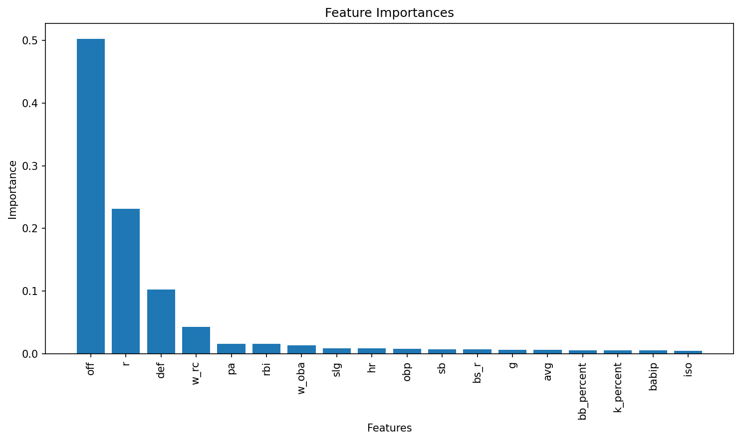

XGBoost

import xgboost as xgb
from xgboost import XGBRegressor, plot_importance
from sklearn.model_selection import GridSearchCV
from sklearn.inspection import PartialDependenceDisplay

# Define the grid of hyperparameters
param_grid = {
    "n_estimators": list(range(20, 201, 20)),  # nrounds: 20, 40, ..., 200
    "learning_rate": [0.025, 0.05, 0.1, 0.3],    # eta
    "gamma": [0],                               # gamma
    "max_depth": [1, 2, 3, 4],
    "colsample_bytree": [1],
    "min_child_weight": [1],
    "subsample": [1]
}

# Initialize the XGBRegressor with the regression objective and fixed random state for reproducibility
xgb_reg = XGBRegressor(objective="reg:squarederror", random_state=1937, verbosity=1)

# Set up GridSearchCV with 10-fold cross-validation; scoring is negative MSE
grid_search = GridSearchCV(
    estimator=xgb_reg,
    param_grid=param_grid,
    scoring="neg_mean_squared_error",
    cv=10,
    verbose=1  # Adjust verbosity as needed
)

# Fit the grid search
grid_search.fit(X_train, y_train)

# Train the final model using the best parameters (grid_search.best_estimator_ is already refit on entire data)
final_model = grid_search.best_estimator_

# Plot variable importance using XGBoost's plot_importance function
plt.figure(figsize=(10, 8))
plot_importance(final_model)
plt.title("Feature Importance")
plt.show()

# Calculate MSE on the training data
y_pred_train = final_model.predict(X_train)
train_mse = mean_squared_error(y_train, y_pred_train)
print("Train MSE:", train_mse)

# Calculate MSE on the test data
y_pred = final_model.predict(X_test)
test_mse = mean_squared_error(y_test, y_pred)
print("Test MSE:", test_mse)

# Print the best parameters found by GridSearchCV
best_params = grid_search.best_params_
print("Best parameters:", best_params)

Fitting 10 folds for each of 160 candidates, totalling 1600 fits

<Figure size 1000x800 with 0 Axes>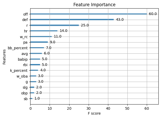

Train MSE: 0.12103999913356943
Test MSE: 0.7061771964936895
Best parameters: {'colsample_bytree': 1, 'gamma': 0, 'learning_rate': 0.3, 'max_depth': 1, 'min_child_weight': 1, 'n_estimators': 200, 'subsample': 1}

# Plot partial dependence for the predictor 'off'
feature_names = mlb_battings_2024.drop(columns=["war"]).columns.tolist()
off_index = feature_names.index("off")
PartialDependenceDisplay.from_estimator(final_model, X_train, features=[off_index],
                                        feature_names=feature_names, kind="average")
plt.title("Partial Dependence for 'off'")
plt.show()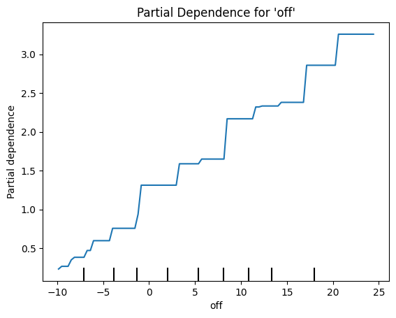

Predictive performance and Overffiting

Train vs. Test MSE for Tree‑Based Models

Model	Train MSE	Test MSE
Regression tree (no depth limit)	0.092	6.154
Regression tree (max_depth = 3)	3.616	7.208
CV‑pruned tree	0.210	5.972
Random forest	0.329	3.332
Gradient boosted tree	0.120	0.706

Predictive Performance Comparison

Unrestricted Regression Tree
- Train MSE: 0.092 (very low)
- Test MSE: 6.154 (high)
- Interpretation: Severe overfitting—model fits noise in training data but generalizes poorly.
Shallow Tree (max_depth = 3)
- Train MSE: 3.616
- Test MSE: 7.208 (highest)
- Interpretation: Underfitting—model is too simple, yielding both high training and test errors.
CV‑Pruned Tree
- Train MSE: 0.210
- Test MSE: 5.972
- Interpretation: Pruning reduces complexity relative to the unrestricted tree, lowering the gap between train and test error but still overfits somewhat.
Random Forest
- Train MSE: 0.329
- Test MSE: 3.332
- Interpretation: Bagging of many trees greatly reduces variance and overfitting compared to single trees, cutting test error by nearly half.
Gradient Boosted Tree
- Train MSE: 0.120
- Test MSE: 0.706 (lowest)
- Interpretation: Sequential boosting captures complex patterns with controlled regularization, achieving the best predictive performance and modest overfit.

Overfitting Analysis

Model	Train MSE	Test MSE	Abs. Difference (Test – Train)
Regression tree (no depth limit)	0.092	6.154	6.062
Regression tree (max_depth = 3)	3.616	7.208	3.592
CV‑pruned tree	0.210	5.972	5.762
Random forest	0.329	3.332	3.003
Gradient boosted tree	0.120	0.706	0.586

Overfit severity can be gauged by the gap between Train and Test MSE:
- Unrestricted tree: gap ≈ 6.062 → very high overfit
- Pruned tree: gap ≈ 5.762 → still substantial overfit
- Random forest: gap ≈ 3.003 → moderate overfit
- Gradient boosted tree: gap ≈ 0.586 → low overfit
Underfitting is evident in the shallow tree (max_depth = 3), which shows both high train and test error.

Overfitting Summary:
- Single trees either overfit (no limit) or underfit (too shallow).
- Pruning helps but does not eliminate overfitting entirely.
- Ensembles (random forest and boosting), particularly boosting, shows a minimal overfit on the test set.