Exam

Supervised Learning

DANL 320: Big Data Analytics, SUNY Geneseo

• Midterm Exam
• Date: April 21, 2025

Honor Pledges

I solemnly swear that I will not cheat or engage in any form of academic dishonesty during this exam.

I will not communicate with other students or use unauthorized materials.

I will uphold the integrity of this exam and demonstrate my own knowledge and abilities.

By taking this pledge, I acknowledge that academic dishonesty undermines the academic process and is a violation of the trust placed in me as a student.

I accept the consequences of any violation of this promise.

• Student’s Name:

Descriptive Statistics

The following provides the descriptive statistics for each part of Exam

    index       part question                             topic  points  mean    sd
0       1        pt1       q1                   VectorAssembler    2.00  0.90  0.21
1       2        NaN       q1       GeneralizedLinearRegression    4.00  0.70  0.26
2       3        NaN       q1                  regression-table    1.00  1.00  0.00
3       4        NaN       q2               prediction-training    1.00  1.00  0.00
4       5        NaN       q2                   prediction-test    1.00  1.00  0.00
5       6        NaN       q3                                ME    2.00  0.95  0.16
6       7        NaN       q4                       ME-year2012    2.00  0.66  0.36
7       8        NaN       q5               double-density-plot    2.00  0.88  0.27
8       9        NaN       q6                         threshold    2.00  0.10  0.32
9      10        NaN       q6                  confusion-matrix    2.00  1.00  0.00
10     11        NaN       q6                          accuracy    0.25  0.90  0.32
11     12        NaN       q6                         precision    0.25  0.90  0.32
12     13        NaN       q6                            recall    0.25  0.90  0.32
13     14        NaN       q6                       specificity    0.25  0.90  0.32
14     15        NaN       q6                      average-rate    0.25  0.90  0.32
15     16        NaN       q6                        enrichment    0.25  0.90  0.32
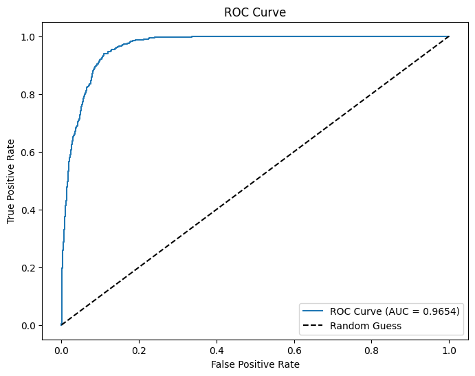
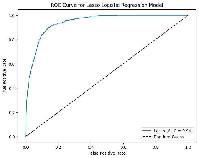
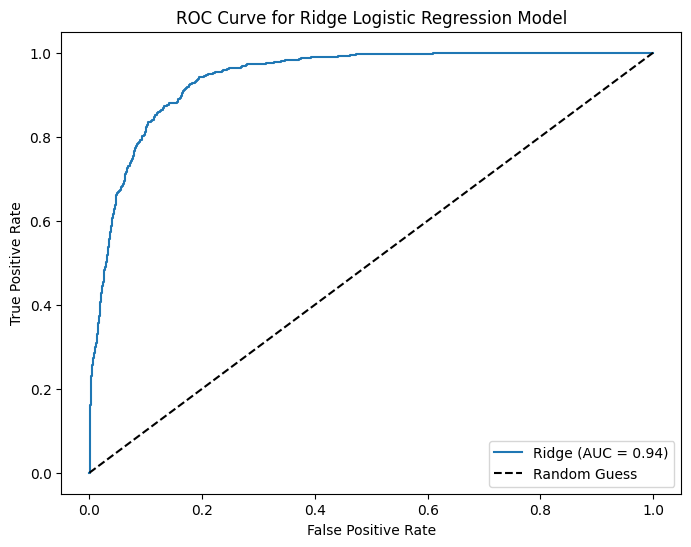
16     17        NaN       q7                               ROC    1.00  0.93  0.24
17     18        NaN       q7                               AUC    1.00  0.93  0.24
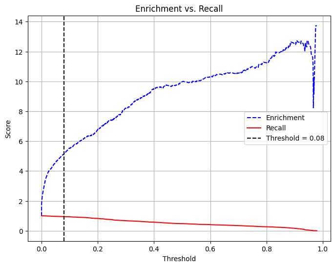
18     19        NaN       q8            recall-enrichment-plot    2.00  0.90  0.32
19     20        NaN       q9   LogisticRegressionCV-penalty=l1    4.00  0.98  0.08
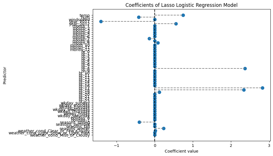
20     21        NaN       q9                        coef_lasso    3.00  1.00  0.00
21     22        NaN       q9                          accuracy    0.25  0.83  0.37
22     23        NaN       q9                         precision    0.25  0.83  0.37
23     24        NaN       q9                            recall    0.25  0.83  0.37
24     25        NaN       q9                               AUC    0.25  0.80  0.42
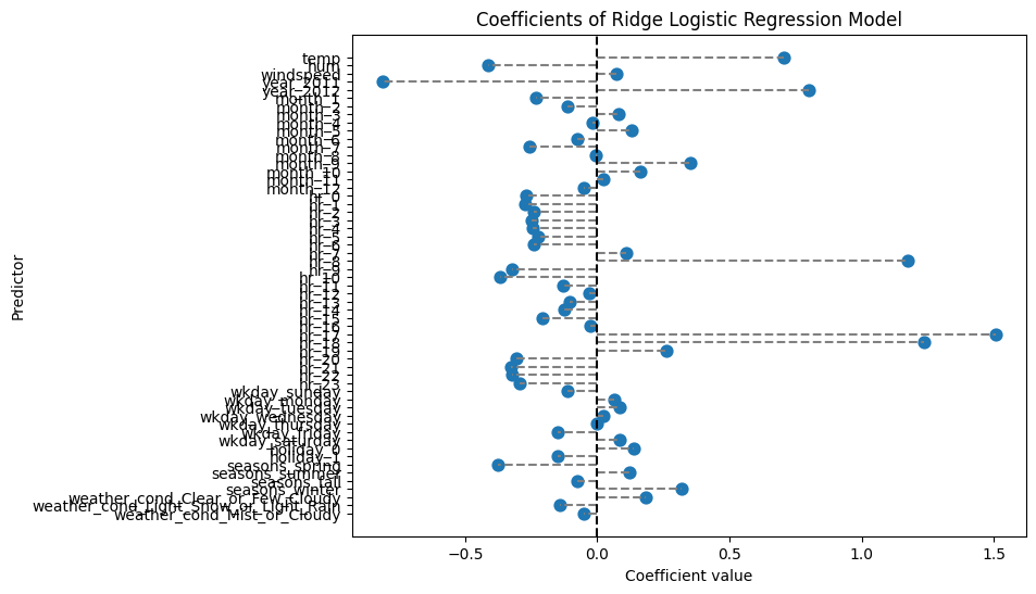
25     26        NaN      q10   LogisticRegressionCV-penalty=l2    1.00  0.88  0.32
26     27        NaN      q10                        coef_ridge    1.00  0.90  0.32
27     28        NaN      q10                          accuracy    0.25  0.80  0.42
28     29        NaN      q10                         precision    0.25  0.80  0.42
29     30        NaN      q10                            recall    0.25  0.80  0.42
30     31        NaN      q10                               AUC    0.25  0.80  0.42
31     32        NaN      q11        DecisionTreeClassifier.fit    4.00  0.50  0.39
32     33        NaN      q11                     max_depth = 6    1.00  0.50  0.53
33     34        NaN      q11      min_impurity_decrease=0.0005    1.00  0.50  0.53
34     35        NaN      q11             min_samples_split=200    1.00  0.53  0.51
35     36        NaN      q11                         plot_tree    2.00  0.45  0.48
36     37        NaN      q12             RandomForestRegressor    4.00  0.85  0.24
37     38        NaN      q12                   max_features=19    1.00  0.60  0.52
38     39        NaN      q12                  n_estimators=500    1.00  1.00  0.00
39     40        NaN      q12                    oob_score=True    1.00  1.00  0.00
40     41        NaN      q12                         Train-MSE    1.00  1.00  0.00
41     42        NaN      q12                          Test-MSE    1.00  1.00  0.00
42     43        NaN      q12                               VIP    2.00  0.60  0.52
43     44        NaN      q13                      XGBRegressor    4.00  1.00  0.00
44     45        NaN      q13                      GridSearchCV    2.00  1.00  0.00
45     46        NaN      q13                               vip    2.00   NaN   NaN
46     47        NaN      q14          PartialDependenceDisplay    3.50  0.70  0.42
47     48  section_2      q15                         beta-temp    1.50  0.54  0.17
48     49        NaN      q15                          beta-hum    1.50  0.00  0.00
49     50        NaN      q15                    beta-year-2012    1.50  0.54  0.17
50     51        NaN      q16                           ME-temp    3.00  0.42  0.42
51     52        NaN      q16                  percentage-point    1.50  0.10  0.32
52     53        NaN      q17                          accuracy    1.00  0.70  0.35
53     54        NaN      q17                         precision    1.00  0.65  0.32
54     55        NaN      q17                            recall    1.00  0.63  0.34
55     56        NaN      q18                             p>1/2    5.00  0.45  0.33
56     57        NaN      q19                        gini/class    2.00  0.53  0.51
57     58        NaN      q19                    decision-rules    3.00  0.65  0.47
58     59        NaN      q20  model-performance-on-unseen-data    3.00  0.78  0.30
59     60        NaN      q20                       overfitting    3.00  0.78  0.34
60     61        NaN     q21a                              bias    2.00  0.20  0.23
61     62        NaN    q21b1                          why-bias    1.00  0.30  0.48
62     63        NaN    q21b2                        cov(x,e)=0    1.00  0.10  0.32
63     64        NaN    q21b3                              when    1.00  0.23  0.42
index                     1
part                    pt1
question                 q1
topic       VectorAssembler
points                  2.0
mean                    0.9
sd                     0.21

Libaries and PySpark Setup

# Below is for an interactive display of Pandas DataFrame in Colab
from google.colab import data_table
data_table.enable_dataframe_formatter()

from tabulate import tabulate  # for table summary

# For basic libraries
import pandas as pd
import numpy as np
import seaborn as sns
import matplotlib.pyplot as plt
import seaborn as sns

import scipy.stats as stats
from scipy.stats import norm
import statsmodels.api as sm  # for lowess smoothing

# `scikit-learn`
from sklearn.metrics import mean_squared_error
from sklearn.metrics import (confusion_matrix, accuracy_score, precision_score, recall_score, roc_curve, roc_auc_score, precision_recall_curve)
from sklearn.model_selection import train_test_split, KFold, cross_val_score
from sklearn.inspection import PartialDependenceDisplay

from sklearn.preprocessing import scale # zero mean & one s.d.
from sklearn.linear_model import LassoCV, lasso_path
from sklearn.linear_model import RidgeCV, Ridge
from sklearn.linear_model import ElasticNetCV
from sklearn.linear_model import LogisticRegression, LogisticRegressionCV

from sklearn.tree import DecisionTreeClassifier, DecisionTreeRegressor, plot_tree
from sklearn.ensemble import RandomForestRegressor
from sklearn.model_selection import GridSearchCV

import xgboost as xgb
from xgboost import XGBRegressor, plot_importance

# PySpark
from pyspark.sql import SparkSession
from pyspark.sql.functions import rand, col, pow, mean, avg, when, log, sqrt, exp
from pyspark.ml.feature import VectorAssembler
from pyspark.ml.regression import LinearRegression, GeneralizedLinearRegression
from pyspark.ml.evaluation import BinaryClassificationEvaluator

spark = SparkSession.builder.master("local[*]").getOrCreate()

UDFs

regression_table()

def regression_table(model, assembler):
    """
    Creates a formatted regression table from a fitted LinearRegression model and its VectorAssembler.

    If the model’s labelCol (retrieved using getLabelCol()) starts with "log", an extra column showing np.exp(coeff)
    is added immediately after the beta estimate column for predictor rows. Additionally, np.exp() of the 95% CI
    Lower and Upper bounds is also added unless the predictor's name includes "log_". The Intercept row does not
    include exponentiated values.

    When labelCol starts with "log", the columns are ordered as:
        y: [label] | Beta | Exp(Beta) | Sig. | Std. Error | p-value | 95% CI Lower | 95% CI Upper | Exp(95% CI Lower) | Exp(95% CI Upper)

    Otherwise, the columns are:
        y: [label] | Beta | Sig. | Std. Error | p-value | 95% CI Lower | 95% CI Upper

    Parameters:
        model: A fitted LinearRegression model (with a .summary attribute and a labelCol).
        assembler: The VectorAssembler used to assemble the features for the model.

    Returns:
        A formatted string containing the regression table.
    """
    # Determine if we should display exponential values for coefficients.
    is_log = model.getLabelCol().lower().startswith("log")

    # Extract coefficients and standard errors as NumPy arrays.
    coeffs = model.coefficients.toArray()
    std_errors_all = np.array(model.summary.coefficientStandardErrors)

    # Check if the intercept's standard error is included (one extra element).
    if len(std_errors_all) == len(coeffs) + 1:
        intercept_se = std_errors_all[0]
        std_errors = std_errors_all[1:]
    else:
        intercept_se = None
        std_errors = std_errors_all

    # Use provided tValues and pValues.
    df = model.summary.numInstances - len(coeffs) - 1
    t_critical = stats.t.ppf(0.975, df)
    p_values = model.summary.pValues

    # Helper: significance stars.
    def significance_stars(p):
        if p < 0.01:
            return "***"
        elif p < 0.05:
            return "**"
        elif p < 0.1:
            return "*"
        else:
            return ""

    # Build table rows for each feature.
    table = []
    for feature, beta, se, p in zip(assembler.getInputCols(), coeffs, std_errors, p_values):
        ci_lower = beta - t_critical * se
        ci_upper = beta + t_critical * se

        # Check if predictor contains "log_" to determine if exponentiation should be applied
        apply_exp = is_log and "log_" not in feature.lower()

        exp_beta = np.exp(beta) if apply_exp else ""
        exp_ci_lower = np.exp(ci_lower) if apply_exp else ""
        exp_ci_upper = np.exp(ci_upper) if apply_exp else ""

        if is_log:
            table.append([
                feature,            # Predictor name
                beta,               # Beta estimate
                exp_beta,           # Exponential of beta (or blank)
                significance_stars(p),
                se,
                p,
                ci_lower,
                ci_upper,
                exp_ci_lower,       # Exponential of 95% CI lower bound
                exp_ci_upper        # Exponential of 95% CI upper bound
            ])
        else:
            table.append([
                feature,
                beta,
                significance_stars(p),
                se,
                p,
                ci_lower,
                ci_upper
            ])

    # Process intercept.
    if intercept_se is not None:
        intercept_p = model.summary.pValues[0] if model.summary.pValues is not None else None
        intercept_sig = significance_stars(intercept_p)
        ci_intercept_lower = model.intercept - t_critical * intercept_se
        ci_intercept_upper = model.intercept + t_critical * intercept_se
    else:
        intercept_sig = ""
        ci_intercept_lower = ""
        ci_intercept_upper = ""
        intercept_se = ""

    if is_log:
        table.append([
            "Intercept",
            model.intercept,
            "",                    # Removed np.exp(model.intercept)
            intercept_sig,
            intercept_se,
            "",
            ci_intercept_lower,
            "",
            ci_intercept_upper,
            ""
        ])
    else:
        table.append([
            "Intercept",
            model.intercept,
            intercept_sig,
            intercept_se,
            "",
            ci_intercept_lower,
            ci_intercept_upper
        ])

    # Append overall model metrics.
    if is_log:
        table.append(["Observations", model.summary.numInstances, "", "", "", "", "", "", "", ""])
        table.append(["R²", model.summary.r2, "", "", "", "", "", "", "", ""])
        table.append(["RMSE", model.summary.rootMeanSquaredError, "", "", "", "", "", "", "", ""])
    else:
        table.append(["Observations", model.summary.numInstances, "", "", "", "", ""])
        table.append(["R²", model.summary.r2, "", "", "", "", ""])
        table.append(["RMSE", model.summary.rootMeanSquaredError, "", "", "", "", ""])

    # Format the table rows.
    formatted_table = []
    for row in table:
        formatted_row = []
        for i, item in enumerate(row):
            # Format Observations as integer with commas.
            if row[0] == "Observations" and i == 1 and isinstance(item, (int, float, np.floating)) and item != "":
                formatted_row.append(f"{int(item):,}")
            elif isinstance(item, (int, float, np.floating)) and item != "":
                if is_log:
                    # When is_log, the columns are:
                    # 0: Metric, 1: Beta, 2: Exp(Beta), 3: Sig, 4: Std. Error, 5: p-value,
                    # 6: 95% CI Lower, 7: 95% CI Upper, 8: Exp(95% CI Lower), 9: Exp(95% CI Upper).
                    if i in [1, 2, 4, 6, 7, 8, 9]:
                        formatted_row.append(f"{item:,.3f}")
                    elif i == 5:
                        formatted_row.append(f"{item:.3f}")
                    else:
                        formatted_row.append(f"{item:.3f}")
                else:
                    # When not is_log, the columns are:
                    # 0: Metric, 1: Beta, 2: Sig, 3: Std. Error, 4: p-value, 5: 95% CI Lower, 6: 95% CI Upper.
                    if i in [1, 3, 5, 6]:
                        formatted_row.append(f"{item:,.3f}")
                    elif i == 4:
                        formatted_row.append(f"{item:.3f}")
                    else:
                        formatted_row.append(f"{item:.3f}")
            else:
                formatted_row.append(item)
        formatted_table.append(formatted_row)

    # Set header and column alignment based on whether label starts with "log"
    if is_log:
        headers = [
            f"y: {model.getLabelCol()}",
            "Beta", "Exp(Beta)", "Sig.", "Std. Error", "p-value",
            "95% CI Lower", "95% CI Upper", "Exp(95% CI Lower)", "Exp(95% CI Upper)"
        ]
        colalign = ("left", "right", "right", "center", "right", "right", "right", "right", "right", "right")
    else:
        headers = [f"y: {model.getLabelCol()}", "Beta", "Sig.", "Std. Error", "p-value", "95% CI Lower", "95% CI Upper"]
        colalign = ("left", "right", "center", "right", "right", "right", "right")

    table_str = tabulate(
        formatted_table,
        headers=headers,
        tablefmt="pretty",
        colalign=colalign
    )

    # Insert a dashed line after the Intercept row.
    lines = table_str.split("\n")
    dash_line = '-' * len(lines[0])
    for i, line in enumerate(lines):
        if "Intercept" in line and not line.strip().startswith('+'):
            lines.insert(i+1, dash_line)
            break

    return "\n".join(lines)

# Example usage:
# print(regression_table(model_1, assembler_1))

add_dummy_variables()

def add_dummy_variables(var_name, reference_level, category_order=None):
    """
    Creates dummy variables for the specified column in the global DataFrames dtrain and dtest.
    Allows manual setting of category order.

    Parameters:
        var_name (str): The name of the categorical column (e.g., "borough_name").
        reference_level (int): Index of the category to be used as the reference (dummy omitted).
        category_order (list, optional): List of categories in the desired order. If None, categories are sorted.

    Returns:
        dummy_cols (list): List of dummy column names excluding the reference category.
        ref_category (str): The category chosen as the reference.
    """
    global dtrain, dtest

    # Get distinct categories from the training set.
    categories = dtrain.select(var_name).distinct().rdd.flatMap(lambda x: x).collect()

    # Convert booleans to strings if present.
    categories = [str(c) if isinstance(c, bool) else c for c in categories]

    # Use manual category order if provided; otherwise, sort categories.
    if category_order:
        # Ensure all categories are present in the user-defined order
        missing = set(categories) - set(category_order)
        if missing:
            raise ValueError(f"These categories are missing from your custom order: {missing}")
        categories = category_order
    else:
        categories = sorted(categories)

    # Validate reference_level
    if reference_level < 0 or reference_level >= len(categories):
        raise ValueError(f"reference_level must be between 0 and {len(categories) - 1}")

    # Define the reference category
    ref_category = categories[reference_level]
    print("Reference category (dummy omitted):", ref_category)

    # Create dummy variables for all categories
    for cat in categories:
        dummy_col_name = var_name + "_" + str(cat).replace(" ", "_")
        dtrain = dtrain.withColumn(dummy_col_name, when(col(var_name) == cat, 1).otherwise(0))
        dtest = dtest.withColumn(dummy_col_name, when(col(var_name) == cat, 1).otherwise(0))

    # List of dummy columns, excluding the reference category
    dummy_cols = [var_name + "_" + str(cat).replace(" ", "_") for cat in categories if cat != ref_category]

    return dummy_cols, ref_category


# Example usage without category_order:
# dummy_cols_year, ref_category_year = add_dummy_variables('year', 0)

# Example usage with category_order:
# custom_order_wkday = ['sunday', 'monday', 'tuesday', 'wednesday', 'thursday', 'friday', 'saturday']
# dummy_cols_wkday, ref_category_wkday = add_dummy_variables('wkday', reference_level=0, category_order = custom_order_wkday)

add_interaction_terms()

def add_interaction_terms(var_list1, var_list2, var_list3=None):
    """
    Creates interaction term columns in the global DataFrames dtrain and dtest.

    For two sets of variable names (which may represent categorical (dummy) or continuous variables),
    this function creates two-way interactions by multiplying each variable in var_list1 with each
    variable in var_list2.

    Optionally, if a third list of variable names (var_list3) is provided, the function also creates
    three-way interactions among each variable in var_list1, each variable in var_list2, and each variable
    in var_list3.

    Parameters:
        var_list1 (list): List of column names for the first set of variables.
        var_list2 (list): List of column names for the second set of variables.
        var_list3 (list, optional): List of column names for the third set of variables for three-way interactions.

    Returns:
        A flat list of new interaction column names.
    """
    global dtrain, dtest

    interaction_cols = []

    # Create two-way interactions between var_list1 and var_list2.
    for var1 in var_list1:
        for var2 in var_list2:
            col_name = f"{var1}_*_{var2}"
            dtrain = dtrain.withColumn(col_name, col(var1).cast("double") * col(var2).cast("double"))
            dtest = dtest.withColumn(col_name, col(var1).cast("double") * col(var2).cast("double"))
            interaction_cols.append(col_name)

    # Create two-way interactions between var_list1 and var_list3.
    if var_list3 is not None:
      for var1 in var_list1:
          for var3 in var_list3:
              col_name = f"{var1}_*_{var3}"
              dtrain = dtrain.withColumn(col_name, col(var1).cast("double") * col(var3).cast("double"))
              dtest = dtest.withColumn(col_name, col(var1).cast("double") * col(var3).cast("double"))
              interaction_cols.append(col_name)

    # Create two-way interactions between var_list2 and var_list3.
    if var_list3 is not None:
      for var2 in var_list2:
          for var3 in var_list3:
              col_name = f"{var2}_*_{var3}"
              dtrain = dtrain.withColumn(col_name, col(var2).cast("double") * col(var3).cast("double"))
              dtest = dtest.withColumn(col_name, col(var2).cast("double") * col(var3).cast("double"))
              interaction_cols.append(col_name)

    # If a third list is provided, create three-way interactions.
    if var_list3 is not None:
        for var1 in var_list1:
            for var2 in var_list2:
                for var3 in var_list3:
                    col_name = f"{var1}_*_{var2}_*_{var3}"
                    dtrain = dtrain.withColumn(col_name, col(var1).cast("double") * col(var2).cast("double") * col(var3).cast("double"))
                    dtest = dtest.withColumn(col_name, col(var1).cast("double") * col(var2).cast("double") * col(var3).cast("double"))
                    interaction_cols.append(col_name)

    return interaction_cols

 # Example
 # interaction_cols_brand_price = add_interaction_terms(dummy_cols_brand, ['log_price'])
 # interaction_cols_brand_ad_price = add_interaction_terms(dummy_cols_brand, dummy_cols_ad, ['log_price'])

compare_reg_models()

def compare_reg_models(models, assemblers, names=None):
    """
    Produces a single formatted table comparing multiple regression models.

    For each predictor (the union across models, ordered by first appearance), the table shows
    the beta estimate (with significance stars) from each model (blank if not used).
    For a predictor, if a model's outcome (model.getLabelCol()) starts with "log", the cell displays
    both the beta and its exponential (separated by " / "), except when the predictor's name includes "log_".
    (The intercept row does not display exp(.))

    Additional rows for Intercept, Observations, R², and RMSE are appended.

    The header's first column is labeled "Predictor", and subsequent columns are
    "y: [outcome] ([name])" for each model.

    The table is produced in grid format (with vertical lines). A dashed line (using '-' characters)
    is inserted at the top, immediately after the header, and at the bottom.
    Additionally, immediately after the Intercept row, the border line is replaced with one using '='
    (to appear as, for example, "+==============================================+==========================+...").

    Parameters:
        models (list): List of fitted LinearRegression models.
        assemblers (list): List of corresponding VectorAssembler objects.
        names (list, optional): List of model names; defaults to "Model 1", "Model 2", etc.

    Returns:
        A formatted string containing the combined regression table.
    """
    # Default model names.
    if names is None:
        names = [f"Model {i+1}" for i in range(len(models))]

    # For each model, get outcome and determine if that model is log-transformed.
    outcomes = [m.getLabelCol() for m in models]
    is_log_flags = [out.lower().startswith("log") for out in outcomes]

    # Build an ordered union of predictors based on first appearance.
    ordered_predictors = []
    for assembler in assemblers:
        for feat in assembler.getInputCols():
            if feat not in ordered_predictors:
                ordered_predictors.append(feat)

    # Helper for significance stars.
    def significance_stars(p):
        if p is None:
            return ""
        if p < 0.01:
            return "***"
        elif p < 0.05:
            return "**"
        elif p < 0.1:
            return "*"
        else:
            return ""

    # Build rows for each predictor.
    rows = []
    for feat in ordered_predictors:
        row = [feat]
        for m, a, is_log in zip(models, assemblers, is_log_flags):
            feats_model = a.getInputCols()
            if feat in feats_model:
                idx = feats_model.index(feat)
                beta = m.coefficients.toArray()[idx]
                p_val = m.summary.pValues[idx] if m.summary.pValues is not None else None
                stars = significance_stars(p_val)
                cell = f"{beta:.3f}{stars}"
                # Only add exp(beta) if model is log and predictor name does NOT include "log_"
                if is_log and ("log_" not in feat.lower()):
                    cell += f" / {np.exp(beta):,.3f}"
                row.append(cell)
            else:
                row.append("")
        rows.append(row)

    # Build intercept row (do NOT compute exp(intercept)).
    intercept_row = ["Intercept"]
    for m in models:
        std_all = np.array(m.summary.coefficientStandardErrors)
        coeffs = m.coefficients.toArray()
        if len(std_all) == len(coeffs) + 1:
            intercept_p = m.summary.pValues[0] if m.summary.pValues is not None else None
        else:
            intercept_p = None
        sig = significance_stars(intercept_p)
        cell = f"{m.intercept:.3f}{sig}"
        intercept_row.append(cell)
    rows.append(intercept_row)

    # Add Observations row.
    obs_row = ["Observations"]
    for m in models:
        obs = m.summary.numInstances
        obs_row.append(f"{int(obs):,}")
    rows.append(obs_row)

    # Add R² row.
    r2_row = ["R²"]
    for m in models:
        r2_row.append(f"{m.summary.r2:.3f}")
    rows.append(r2_row)

    # Add RMSE row.
    rmse_row = ["RMSE"]
    for m in models:
        rmse_row.append(f"{m.summary.rootMeanSquaredError:.3f}")
    rows.append(rmse_row)

    # Build header: first column "Predictor", then for each model: "y: [outcome] ([name])"
    header = ["Predictor"]
    for out, name in zip(outcomes, names):
        header.append(f"y: {out} ({name})")

    # Create table string using grid format.
    table_str = tabulate(rows, headers=header, tablefmt="grid", colalign=("left",) + ("right",)*len(models))

    # Split into lines.
    lines = table_str.split("\n")

    # Create a dashed line spanning the full width.
    full_width = len(lines[0])
    dash_line = '-' * full_width
    # Create an equals line by replacing '-' with '='.
    eq_line = dash_line.replace('-', '=')

    # Insert a dashed line after the header row.
    lines = table_str.split("\n")
    # In grid format, header and separator are usually the first two lines.
    lines.insert(2, dash_line)

    # Insert an equals line after the Intercept row.
    for i, line in enumerate(lines):
        if line.startswith("|") and "Intercept" in line:
            if i+1 < len(lines):
                lines[i+1] = eq_line
            break

    # Add dashed lines at the very top and bottom.
    final_table = dash_line + "\n" + "\n".join(lines) + "\n" + dash_line

    return final_table

# Example usage:
# print(compare_reg_models([model_1, model_2, model_3],
#                          [assembler_1, assembler_2, assembler_3],
#                          ["Model 1", "Model 2", "Model 3"]))

compare_rmse()

def compare_rmse(test_dfs, label_col, pred_col="prediction", names=None):
    """
    Computes and compares RMSE values for a list of test DataFrames.

    For each DataFrame in test_dfs, this function calculates the RMSE between the actual outcome
    (given by label_col) and the predicted value (given by pred_col, default "prediction"). It then
    produces a formatted table where the first column header is empty and the first row's first cell is
    "RMSE", with each model's RMSE in its own column.

    Parameters:
        test_dfs (list): List of test DataFrames.
        label_col (str): The name of the outcome column.
        pred_col (str, optional): The name of the prediction column (default "prediction").
        names (list, optional): List of model names corresponding to the test DataFrames.
                                Defaults to "Model 1", "Model 2", etc.

    Returns:
        A formatted string containing a table that compares RMSE values for each test DataFrame,
        with one model per column.
    """
    # Set default model names if none provided.
    if names is None:
        names = [f"Model {i+1}" for i in range(len(test_dfs))]

    rmse_values = []
    for df in test_dfs:
        # Create a column for squared error.
        df = df.withColumn("error_sq", pow(col(label_col) - col(pred_col), 2))
        # Calculate RMSE: square root of the mean squared error.
        rmse = df.agg(sqrt(avg("error_sq")).alias("rmse")).collect()[0]["rmse"]
        rmse_values.append(rmse)

    # Build a single row table: first cell "RMSE", then one cell per model with the RMSE value.
    row = ["RMSE"] + [f"{rmse:.3f}" for rmse in rmse_values]

    # Build header: first column header is empty, then model names.
    header = [""] + names

    table_str = tabulate([row], headers=header, tablefmt="grid", colalign=("left",) + ("right",)*len(names))
    return table_str

# Example usage:
# print(compare_rmse([dtest_1, dtest_2, dtest_3], "log_sales", names=["Model 1", "Model 2", "Model 3"]))

residual_plot()

def residual_plot(df, label_col, model_name):
    """
    Generates a residual plot for a given test dataframe.

    Parameters:
        df (DataFrame): Spark DataFrame containing the test set with predictions.
        label_col (str): The column name of the actual outcome variable.
        title (str): The title for the residual plot.

    Returns:
        None (displays the plot)
    """
    # Convert to Pandas DataFrame
    df_pd = df.select(["prediction", label_col]).toPandas()
    df_pd["residual"] = df_pd[label_col] - df_pd["prediction"]

    # Scatter plot of residuals vs. predicted values
    plt.scatter(df_pd["prediction"], df_pd["residual"], alpha=0.2, color="darkgray")

    # Use LOWESS smoothing for trend line
    smoothed = sm.nonparametric.lowess(df_pd["residual"], df_pd["prediction"])
    plt.plot(smoothed[:, 0], smoothed[:, 1], color="darkblue")

    # Add reference line at y=0
    plt.axhline(y=0, color="red", linestyle="--")

    # Labels and title (model_name)
    plt.xlabel("Predicted Values")
    plt.ylabel("Residuals")
    model_name = "Residual Plot for " + model_name
    plt.title(model_name)

    # Show plot
    plt.show()

# Example usage:
# residual_plot(dtest_1, "log_sales", "Model 1")

marginal_effects()

def marginal_effects(model, means):
    """
    Compute marginal effects for all predictors in a PySpark GeneralizedLinearRegression model (logit)
    and return a formatted table with statistical significance and standard errors.

    Parameters:
        model: Fitted GeneralizedLinearRegression model (with binomial family and logit link).
        means: List of mean values for the predictor variables.

    Returns:
        - A formatted string containing the marginal effects table.
        - A Pandas DataFrame with marginal effects, standard errors, confidence intervals, and significance stars.
    """
    global assembler_predictors  # Use the global assembler_predictors list

    # Extract model coefficients, standard errors, and intercept
    coeffs = np.array(model.coefficients)
    std_errors = np.array(model.summary.coefficientStandardErrors)
    intercept = model.intercept

    # Compute linear combination of means and coefficients (XB)
    XB = np.dot(means, coeffs) + intercept

    # Compute derivative of logistic function (G'(XB))
    G_prime_XB = np.exp(XB) / ((1 + np.exp(XB)) ** 2)

    # Helper: significance stars.
    def significance_stars(p):
        if p < 0.01:
            return "***"
        elif p < 0.05:
            return "**"
        elif p < 0.1:
            return "*"
        else:
            return ""

    # Create lists to store results
    results = []
    df_results = []  # For Pandas DataFrame

    for i, predictor in enumerate(assembler_predictors):
        # Compute marginal effect
        marginal_effect = G_prime_XB * coeffs[i]

        # Compute standard error of the marginal effect
        std_error = G_prime_XB * std_errors[i]

        # Compute z-score and p-value
        z_score = marginal_effect / std_error if std_error != 0 else np.nan
        p_value = 2 * (1 - norm.cdf(abs(z_score))) if not np.isnan(z_score) else np.nan

        # Compute confidence interval (95%)
        ci_lower = marginal_effect - 1.96 * std_error
        ci_upper = marginal_effect + 1.96 * std_error

        # Append results for table formatting
        results.append([
            predictor,
            f"{marginal_effect: .6f}",
            significance_stars(p_value),
            f"{std_error: .6f}",
            f"{ci_lower: .6f}",
            f"{ci_upper: .6f}"
        ])

        # Append results for Pandas DataFrame
        df_results.append({
            "Variable": predictor,
            "Marginal Effect": marginal_effect,
            "Significance": significance_stars(p_value),
            "Std. Error": std_error,
            "95% CI Lower": ci_lower,
            "95% CI Upper": ci_upper
        })

    # Convert results to formatted table
    table_str = tabulate(results, headers=["Variable", "Marginal Effect", "Significance", "Std. Error", "95% CI Lower", "95% CI Upper"],
                         tablefmt="pretty", colalign=("left", "decimal", "left", "decimal", "decimal", "decimal"))

    # Convert results to Pandas DataFrame
    df_results = pd.DataFrame(df_results)

    return table_str, df_results

# Example usage:
# means = [0.5, 30]  # Mean values for x1 and x2
# assembler_predictors = ['x1', 'x2']  # Define globally before calling the function
# table_output, df_output = marginal_effects(fitted_model, means)
# print(table_output)
# display(df_output)

Section 1. Bikeshare in D.C.

Data Preparation

# 1. Read CSV data from URL
df_pd = pd.read_csv('https://bcdanl.github.io/data/bikeshare_cleaned.csv')

# Adding an `over_load` variable
df_pd['over_load'] = np.where(df_pd['cnt'] > 500, 1, 0)

df_pd

	cnt	year	month	date	hr	wkday	holiday	seasons	weather_cond	temp	hum	windspeed	over_load
0	16	2011	1	1	0	saturday	0	spring	Clear or Few Cloudy	-1.334609	0.947345	-1.553844	0
1	40	2011	1	1	1	saturday	0	spring	Clear or Few Cloudy	-1.438475	0.895513	-1.553844	0
2	32	2011	1	1	2	saturday	0	spring	Clear or Few Cloudy	-1.438475	0.895513	-1.553844	0
3	13	2011	1	1	3	saturday	0	spring	Clear or Few Cloudy	-1.334609	0.636351	-1.553844	0
4	1	2011	1	1	4	saturday	0	spring	Clear or Few Cloudy	-1.334609	0.636351	-1.553844	0
...	...	...	...	...	...	...	...	...	...	...	...	...	...
17371	119	2012	12	31	19	monday	0	spring	Mist or Cloudy	-1.230743	-0.141133	-0.211685	0
17372	89	2012	12	31	20	monday	0	spring	Mist or Cloudy	-1.230743	-0.141133	-0.211685	0
17373	90	2012	12	31	21	monday	0	spring	Clear or Few Cloudy	-1.230743	-0.141133	-0.211685	0
17374	61	2012	12	31	22	monday	0	spring	Clear or Few Cloudy	-1.230743	-0.348463	-0.456086	0
17375	49	2012	12	31	23	monday	0	spring	Clear or Few Cloudy	-1.230743	0.118028	-0.456086	0

17376 rows × 13 columns

Variable description

Variable	Description
cnt	Count of total rental bikes
year	Year
month	Month
date	Date
hr	Hour
wkday	Weekday
holiday	Holiday indicator (1 if holiday, 0 otherwise)
seasons	Season
weather_cond	Weather condition
temp	Temperature (measured in standard deviations from average)
hum	Humidity (measured in standard deviations from average)
windspeed	Wind speed (measured in standard deviations from average)
over_load	1 if `cnt > 500; 0 otherwise

# 2. Convert pandas DataFrame into PySpark DataFrame
df = spark.createDataFrame(df_pd)

# 3. Train-test split
dtrain, dtest = df.randomSplit([0.6, 0.4], seed = 1234)

# 4. Adding Dummies
dummy_cols_year, ref_category_year = add_dummy_variables('year', 0)
dummy_cols_month, ref_category_month = add_dummy_variables('month', 0)
dummy_cols_hr, ref_category_hr = add_dummy_variables('hr', 0)

custom_order_wkday = ['sunday', 'monday', 'tuesday', 'wednesday', 'thursday', 'friday', 'saturday'] # Custom category_order
dummy_cols_wkday, ref_category_wkday = add_dummy_variables('wkday', reference_level=0, category_order = custom_order_wkday)

dummy_cols_holiday, ref_category_holiday = add_dummy_variables('holiday', 0)

custom_order_seasons = ['spring', 'summer', 'fall', 'winter']  # Custom category_order
dummy_cols_seasons, ref_category_seasons = add_dummy_variables('seasons', 0, custom_order_seasons)

dummy_cols_weather_cond, ref_category_weather_cond = add_dummy_variables('weather_cond', 0)

Reference category (dummy omitted): 2011
Reference category (dummy omitted): 1
Reference category (dummy omitted): 0
Reference category (dummy omitted): sunday
Reference category (dummy omitted): 0
Reference category (dummy omitted): spring
Reference category (dummy omitted): Clear or Few Cloudy

Question 1

Fit the following logistic regression model:

\[ \begin{align} \text{Prob}(\text{over\_load}_{i} = 1) =\ G\Big(&\beta_{\text{intercept}}\\ &+ \beta_{\text{temp}} \, \text{temp}_{i} + \beta_{\text{hum}} \, \text{hum}_{i} + \beta_{\text{windspeed}} \, \text{windspeed}_{i} \nonumber \\ &+ \beta_{\text{year\_2012}} \, \text{year\_2012}_{i}\\ &+ \beta_{\text{month\_2}} \, \text{month\_2}_{i} + \beta_{\text{month\_3}} \, \text{month\_3}_{i} + \beta_{\text{month\_4}} \, \text{month\_4}_{i} \nonumber \\ &+ \beta_{\text{month\_5}} \, \text{month\_5}_{i} + \beta_{\text{month\_6}} \, \text{month\_6}_{i} + \beta_{\text{month\_7}} \, \text{month\_7}_{i} + \beta_{\text{month\_8}} \, \text{month\_8}_{i} \nonumber \\ &+ \beta_{\text{month\_9}} \, \text{month\_9}_{i} + \beta_{\text{month\_10}} \, \text{month\_10}_{i} + \beta_{\text{month\_11}} \, \text{month\_11}_{i} + \beta_{\text{month\_12}} \, \text{month\_12}_{i} \nonumber \\ &+ \beta_{\text{hr\_1}} \, \text{hr\_1}_{i} + \beta_{\text{hr\_2}} \, \text{hr\_2}_{i} + \beta_{\text{hr\_3}} \, \text{hr\_3}_{i} + \beta_{\text{hr\_4}} \, \text{hr\_4}_{i} \nonumber \\ &+ \beta_{\text{hr\_5}} \, \text{hr\_5}_{i} + \beta_{\text{hr\_6}} \, \text{hr\_6}_{i} + \beta_{\text{hr\_7}} \, \text{hr\_7}_{i} + \beta_{\text{hr\_8}} \, \text{hr\_8}_{i} \nonumber \\ &+ \beta_{\text{hr\_9}} \, \text{hr\_9}_{i} + \beta_{\text{hr\_10}} \, \text{hr\_10}_{i} + \beta_{\text{hr\_11}} \, \text{hr\_11}_{i} + \beta_{\text{hr\_12}} \, \text{hr\_12}_{i} \nonumber \\ &+ \beta_{\text{hr\_13}} \, \text{hr\_13}_{i} + \beta_{\text{hr\_14}} \, \text{hr\_14}_{i} + \beta_{\text{hr\_15}} \, \text{hr\_15}_{i} + \beta_{\text{hr\_16}} \, \text{hr\_16}_{i} \nonumber \\ &+ \beta_{\text{hr\_17}} \, \text{hr\_17}_{i} + \beta_{\text{hr\_18}} \, \text{hr\_18}_{i} + \beta_{\text{hr\_19}} \, \text{hr\_19}_{i} + \beta_{\text{hr\_20}} \, \text{hr\_20}_{i} \nonumber \\ &+ \beta_{\text{hr\_21}} \, \text{hr\_21}_{i} + \beta_{\text{hr\_22}} \, \text{hr\_22}_{i} + \beta_{\text{hr\_23}} \, \text{hr\_23}_{i} \nonumber \\ &+ \beta_{\text{wkday\_monday}} \, \text{wkday\_monday}_{i} + \beta_{\text{wkday\_tuesday}} \, \text{wkday\_tuesday}_{i} + \beta_{\text{wkday\_wednesday}} \, \text{wkday\_wednesday}_{i} \nonumber \\ &+ \beta_{\text{wkday\_thursday}} \, \text{wkday\_thursday}_{i} + \beta_{\text{wkday\_friday}} \, \text{wkday\_friday}_{i} + \beta_{\text{wkday\_saturday}} \, \text{wkday\_saturday}_{i} \nonumber \\ &+ \beta_{\text{holiday\_1}} \, \text{holiday\_1}_{i} \nonumber \\ &+ \beta_{\text{seasons\_summer}} \, \text{seasons\_summer}_{i} + \beta_{\text{seasons\_fall}} \, \text{seasons\_fall}_{i} + \beta_{\text{seasons\_winter}} \, \text{seasons\_winter}_{i} \nonumber \\ &+ \beta_{\text{weather\_cond\_Light\_Snow\_or\_Light\_Rain}} \, \text{weather\_cond\_Light\_Snow\_or\_Light\_Rain}_{i}\nonumber \\ &+ \beta_{\text{weather\_cond\_Mist\_or\_Cloudy}} \, \text{weather\_cond\_Mist\_or\_Cloudy}_{i}\Big) \end{align} \]

where \(G(\,\cdot\,)\) is

\[ G(\,\cdot\,) = \frac{\exp(\,\cdot\,)}{1 + \exp(\,\cdot\,)}. \]

# assembling predictors
conti_cols = ["temp", "hum", "windspeed"]

# Keep the name assembler_predictors unchanged,
#   as it will be used as a global variable in the marginal_effects UDF.
assembler_predictors = (
    conti_cols +
    dummy_cols_year +
    dummy_cols_month +
    dummy_cols_hr +
    dummy_cols_wkday +
    dummy_cols_holiday +
    dummy_cols_seasons +
    dummy_cols_weather_cond
)

assembler_1 = VectorAssembler(
    inputCols = assembler_predictors,
    outputCol = "predictors"
)

dtrain_1 = assembler_1.transform(dtrain)
dtest_1  = assembler_1.transform(dtest)


# training the model
model_1 = (
    GeneralizedLinearRegression(featuresCol="predictors",
                                labelCol="over_load",
                                family="binomial",
                                link="logit")
    .fit(dtrain_1)
)

Question 2

• Make a prediction on training data
• Make a prediction on test data

# making prediction on both training and test
dtrain_1 = model_1.transform(dtrain_1)
dtest_1 = model_1.transform(dtest_1)

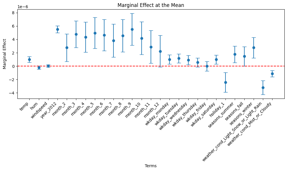
Question 3

• Calculate the marginal effect of each predictor at the mean.

# Compute means
means_df = dtrain_1.select([mean(col).alias(col) for col in assembler_predictors])

# Collect the results as a list
means = means_df.collect()[0]
means_list = [means[col] for col in assembler_predictors]
table_output, df_ME = marginal_effects(model_1, means_list) # Instead of mean values, some other representative values can also be chosen.
print(table_output)

+---------------------------------------+-----------------+--------------+------------+--------------+--------------+
| Variable                              | Marginal Effect | Significance | Std. Error | 95% CI Lower | 95% CI Upper |
+---------------------------------------+-----------------+--------------+------------+--------------+--------------+
| temp                                  |        0.000001 | ***          |   0.000000 |     0.000001 |     0.000001 |
| hum                                   |       -0.000000 |              |   0.000000 |    -0.000000 |     0.000000 |
| windspeed                             |        0.000000 |              |   0.000000 |    -0.000000 |     0.000000 |
| year_2012                             |        0.000006 | ***          |   0.000000 |     0.000005 |     0.000006 |
| month_2                               |        0.000003 | ***          |   0.000001 |     0.000001 |     0.000005 |
| month_3                               |        0.000005 | ***          |   0.000001 |     0.000003 |     0.000007 |
| month_4                               |        0.000004 | ***          |   0.000001 |     0.000002 |     0.000007 |
| month_5                               |        0.000005 | ***          |   0.000001 |     0.000003 |     0.000007 |
| month_6                               |        0.000005 | ***          |   0.000001 |     0.000002 |     0.000007 |
| month_7                               |        0.000004 | ***          |   0.000001 |     0.000001 |     0.000006 |
| month_8                               |        0.000005 | ***          |   0.000001 |     0.000002 |     0.000007 |
| month_9                               |        0.000006 | ***          |   0.000001 |     0.000003 |     0.000008 |
| month_10                              |        0.000004 | ***          |   0.000001 |     0.000002 |     0.000007 |
| month_11                              |        0.000003 | **           |   0.000001 |     0.000000 |     0.000005 |
| month_12                              |        0.000002 | *            |   0.000001 |    -0.000000 |     0.000005 |
| hr_1                                  |       -0.000000 |              |   0.036195 |    -0.070942 |     0.070941 |
| hr_2                                  |       -0.000000 |              |   0.036280 |    -0.071109 |     0.071109 |
| hr_3                                  |       -0.000000 |              |   0.036581 |    -0.071698 |     0.071698 |
| hr_4                                  |       -0.000000 |              |   0.036064 |    -0.070685 |     0.070685 |
| hr_5                                  |       -0.000000 |              |   0.036315 |    -0.071177 |     0.071177 |
| hr_6                                  |       -0.000000 |              |   0.036108 |    -0.070772 |     0.070772 |
| hr_7                                  |        0.000040 |              |   0.025399 |    -0.049742 |     0.049823 |
| hr_8                                  |        0.000045 |              |   0.025399 |    -0.049738 |     0.049827 |
| hr_9                                  |       -0.000000 |              |   0.035986 |    -0.070534 |     0.070533 |
| hr_10                                 |        0.000034 |              |   0.025399 |    -0.049749 |     0.049816 |
| hr_11                                 |        0.000039 |              |   0.025399 |    -0.049743 |     0.049822 |
| hr_12                                 |        0.000040 |              |   0.025399 |    -0.049742 |     0.049823 |
| hr_13                                 |        0.000040 |              |   0.025399 |    -0.049742 |     0.049822 |
| hr_14                                 |        0.000040 |              |   0.025399 |    -0.049743 |     0.049822 |
| hr_15                                 |        0.000039 |              |   0.025399 |    -0.049743 |     0.049822 |
| hr_16                                 |        0.000040 |              |   0.025399 |    -0.049742 |     0.049823 |
| hr_17                                 |        0.000046 |              |   0.025399 |    -0.049736 |     0.049829 |
| hr_18                                 |        0.000045 |              |   0.025399 |    -0.049737 |     0.049828 |
| hr_19                                 |        0.000042 |              |   0.025399 |    -0.049741 |     0.049824 |
| hr_20                                 |        0.000037 |              |   0.025399 |    -0.049745 |     0.049819 |
| hr_21                                 |        0.000034 |              |   0.025399 |    -0.049748 |     0.049817 |
| hr_22                                 |        0.000034 |              |   0.025399 |    -0.049748 |     0.049816 |
| hr_23                                 |       -0.000000 |              |   0.035965 |    -0.070491 |     0.070491 |
| wkday_monday                          |        0.000001 | ***          |   0.000000 |     0.000000 |     0.000002 |
| wkday_tuesday                         |        0.000001 | ***          |   0.000000 |     0.000000 |     0.000002 |
| wkday_wednesday                       |        0.000001 | ***          |   0.000000 |     0.000000 |     0.000002 |
| wkday_thursday                        |        0.000001 | *            |   0.000000 |    -0.000000 |     0.000001 |
| wkday_friday                          |       -0.000000 |              |   0.000000 |    -0.000001 |     0.000001 |
| wkday_saturday                        |        0.000001 | ***          |   0.000000 |     0.000000 |     0.000002 |
| holiday_1                             |       -0.000002 | ***          |   0.000001 |    -0.000004 |    -0.000001 |
| seasons_summer                        |        0.000002 | ***          |   0.000001 |     0.000001 |     0.000003 |
| seasons_fall                          |        0.000001 | **           |   0.000001 |     0.000000 |     0.000003 |
| seasons_winter                        |        0.000003 | ***          |   0.000001 |     0.000001 |     0.000004 |
| weather_cond_Light_Snow_or_Light_Rain |       -0.000003 | ***          |   0.000001 |    -0.000004 |    -0.000002 |
| weather_cond_Mist_or_Cloudy           |       -0.000001 | ***          |   0.000000 |    -0.000002 |    -0.000001 |
+---------------------------------------+-----------------+--------------+------------+--------------+--------------+

df_ME2 = df_ME[~df_ME['Variable'].str.contains('hr_')]

# Increase figure size to prevent overlapping
plt.figure(figsize=(10, 6))

# Plot using the DataFrame columns
plt.errorbar(df_ME2["Variable"], df_ME2["Marginal Effect"],
             yerr=1.96 * df_ME2["Std. Error"], fmt='o', capsize=5)

# Labels and title
plt.xlabel("Terms")
plt.ylabel("Marginal Effect")
plt.title("Marginal Effect at the Mean")

# Add horizontal line at 0 for reference
plt.axhline(0, color="red", linestyle="--")

# Adjust x-axis labels to avoid overlap
plt.xticks(rotation=45, ha="right")  # Rotate and align labels to the right
plt.tight_layout()  # Adjust layout to prevent overlap

# Show plot
plt.show()

Question 4

• Calculate the marginal effect of each predictor at the mean for year 2012.

# Compute means for year2012
means_df_year2012 = (
    dtrain_1
    .filter(
        ( col("year_2012") == 1 )
    )
    .select([mean(col).alias(col) for col in assembler_predictors])
)

# Collect the results as a list
means_year2012 = means_df_year2012.collect()[0]
means_list_year2012 = [means_year2012[col] for col in assembler_predictors]

table_output_s, df_ME_s = marginal_effects(model_1, means_list_year2012) # Instead of mean values, some other representative values can also be chosen.
print(table_output_s)

+---------------------------------------+-----------------+--------------+------------+--------------+--------------+
| Variable                              | Marginal Effect | Significance | Std. Error | 95% CI Lower | 95% CI Upper |
+---------------------------------------+-----------------+--------------+------------+--------------+--------------+
| temp                                  |        0.000005 | ***          |   0.000001 |     0.000003 |     0.000008 |
| hum                                   |       -0.000001 |              |   0.000001 |    -0.000002 |     0.000000 |
| windspeed                             |        0.000000 |              |   0.000001 |    -0.000001 |     0.000001 |
| year_2012                             |        0.000029 | ***          |   0.000001 |     0.000027 |     0.000032 |
| month_2                               |        0.000015 | ***          |   0.000006 |     0.000004 |     0.000026 |
| month_3                               |        0.000025 | ***          |   0.000005 |     0.000015 |     0.000036 |
| month_4                               |        0.000023 | ***          |   0.000006 |     0.000011 |     0.000035 |
| month_5                               |        0.000026 | ***          |   0.000006 |     0.000014 |     0.000039 |
| month_6                               |        0.000025 | ***          |   0.000006 |     0.000012 |     0.000037 |
| month_7                               |        0.000020 | ***          |   0.000007 |     0.000007 |     0.000034 |
| month_8                               |        0.000024 | ***          |   0.000007 |     0.000011 |     0.000037 |
| month_9                               |        0.000029 | ***          |   0.000006 |     0.000017 |     0.000042 |
| month_10                              |        0.000022 | ***          |   0.000007 |     0.000009 |     0.000035 |
| month_11                              |        0.000015 | **           |   0.000007 |     0.000002 |     0.000028 |
| month_12                              |        0.000012 | *            |   0.000006 |    -0.000001 |     0.000025 |
| hr_1                                  |       -0.000001 |              |   0.192744 |    -0.377779 |     0.377776 |
| hr_2                                  |       -0.000000 |              |   0.193199 |    -0.378670 |     0.378669 |
| hr_3                                  |       -0.000001 |              |   0.194799 |    -0.381807 |     0.381805 |
| hr_4                                  |       -0.000001 |              |   0.192047 |    -0.376413 |     0.376412 |
| hr_5                                  |       -0.000000 |              |   0.193384 |    -0.379032 |     0.379032 |
| hr_6                                  |       -0.000000 |              |   0.192284 |    -0.376876 |     0.376876 |
| hr_7                                  |        0.000214 |              |   0.135256 |    -0.264887 |     0.265315 |
| hr_8                                  |        0.000237 |              |   0.135256 |    -0.264864 |     0.265339 |
| hr_9                                  |       -0.000002 |              |   0.191634 |    -0.375605 |     0.375602 |
| hr_10                                 |        0.000180 |              |   0.135256 |    -0.264921 |     0.265281 |
| hr_11                                 |        0.000210 |              |   0.135256 |    -0.264891 |     0.265311 |
| hr_12                                 |        0.000214 |              |   0.135256 |    -0.264887 |     0.265315 |
| hr_13                                 |        0.000213 |              |   0.135256 |    -0.264888 |     0.265314 |
| hr_14                                 |        0.000212 |              |   0.135256 |    -0.264889 |     0.265313 |
| hr_15                                 |        0.000210 |              |   0.135256 |    -0.264891 |     0.265311 |
| hr_16                                 |        0.000215 |              |   0.135256 |    -0.264886 |     0.265316 |
| hr_17                                 |        0.000248 |              |   0.135256 |    -0.264853 |     0.265349 |
| hr_18                                 |        0.000241 |              |   0.135256 |    -0.264860 |     0.265343 |
| hr_19                                 |        0.000221 |              |   0.135256 |    -0.264880 |     0.265322 |
| hr_20                                 |        0.000197 |              |   0.135256 |    -0.264904 |     0.265298 |
| hr_21                                 |        0.000182 |              |   0.135256 |    -0.264919 |     0.265283 |
| hr_22                                 |        0.000181 |              |   0.135256 |    -0.264920 |     0.265282 |
| hr_23                                 |       -0.000001 |              |   0.191520 |    -0.375381 |     0.375378 |
| wkday_monday                          |        0.000005 | ***          |   0.000002 |     0.000002 |     0.000009 |
| wkday_tuesday                         |        0.000006 | ***          |   0.000002 |     0.000003 |     0.000010 |
| wkday_wednesday                       |        0.000005 | ***          |   0.000002 |     0.000001 |     0.000009 |
| wkday_thursday                        |        0.000003 | *            |   0.000002 |    -0.000001 |     0.000007 |
| wkday_friday                          |       -0.000000 |              |   0.000002 |    -0.000004 |     0.000004 |
| wkday_saturday                        |        0.000005 | ***          |   0.000002 |     0.000002 |     0.000009 |
| holiday_1                             |       -0.000013 | ***          |   0.000004 |    -0.000021 |    -0.000005 |
| seasons_summer                        |        0.000009 | ***          |   0.000003 |     0.000003 |     0.000016 |
| seasons_fall                          |        0.000008 | **           |   0.000004 |     0.000000 |     0.000016 |
| seasons_winter                        |        0.000015 | ***          |   0.000004 |     0.000006 |     0.000023 |
| weather_cond_Light_Snow_or_Light_Rain |       -0.000017 | ***          |   0.000003 |    -0.000023 |    -0.000011 |
| weather_cond_Mist_or_Cloudy           |       -0.000006 | ***          |   0.000001 |    -0.000009 |    -0.000003 |
+---------------------------------------+-----------------+--------------+------------+--------------+--------------+

df_ME_s2 = df_ME_s[~df_ME_s['Variable'].str.contains('hr_')]

# Increase figure size to prevent overlapping
plt.figure(figsize=(10, 6))

# Plot using the DataFrame columns
plt.errorbar(df_ME_s2["Variable"], df_ME_s2["Marginal Effect"],
             yerr=1.96 * df_ME_s2["Std. Error"], fmt='o', capsize=5)

# Labels and title
plt.xlabel("Terms")
plt.ylabel("Marginal Effect")
plt.title("Marginal Effect at the Mean")

# Add horizontal line at 0 for reference
plt.axhline(0, color="red", linestyle="--")

# Adjust x-axis labels to avoid overlap
plt.xticks(rotation=45, ha="right")  # Rotate and align labels to the right
plt.tight_layout()  # Adjust layout to prevent overlap

# Show plot
plt.show()

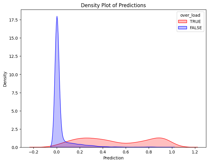
Question 5

Visualize a double density plot of predictions

# Filter training data for atRisk == 1 and atRisk == 0
pdf = dtrain_1.select("prediction", "over_load").toPandas()

train_true = pdf[pdf["over_load"] == 1]
train_false = pdf[pdf["over_load"] == 0]

# Create the first density plot
plt.figure(figsize=(8, 6))
sns.kdeplot(train_true["prediction"], label="TRUE", color="red", fill=True)
sns.kdeplot(train_false["prediction"], label="FALSE", color="blue", fill=True)
plt.xlabel("Prediction")
plt.ylabel("Density")
plt.title("Density Plot of Predictions")
plt.legend(title="over_load")
plt.show()

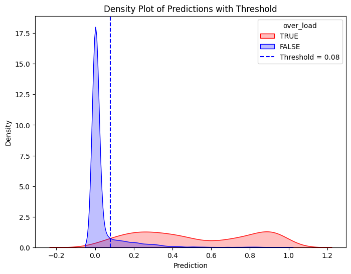
# Define threshold for vertical line
threshold = 0.08  # Replace with actual value

# Create the second density plot with vertical line
plt.figure(figsize=(8, 6))
sns.kdeplot(train_true["prediction"], label="TRUE", color="red", fill=True)
sns.kdeplot(train_false["prediction"], label="FALSE", color="blue", fill=True)
plt.axvline(x=threshold, color="blue", linestyle="dashed", label=f"Threshold = {threshold}")
plt.xlabel("Prediction")
plt.ylabel("Density")
plt.title("Density Plot of Predictions with Threshold")
plt.legend(title="over_load")
plt.show()

Question 6

• Calculate the followings:
  • Confusion matrix with the threshold level that clearly separates the double density plots
  • Accuracy
  • Precision
  • Recall
  • Specificity
  • Average rate of at-risk babies
  • Enrichment

# Compute confusion matrix
dtest_1 = dtest_1.withColumn("predicted_class", when(col("prediction") > threshold, 1).otherwise(0))
conf_matrix = dtest_1.groupBy("over_load", "predicted_class").count().orderBy("over_load", "predicted_class")

TP = dtest_1.filter((col("over_load") == 1) & (col("predicted_class") == 1)).count()
FP = dtest_1.filter((col("over_load") == 0) & (col("predicted_class") == 1)).count()
FN = dtest_1.filter((col("over_load") == 1) & (col("predicted_class") == 0)).count()
TN = dtest_1.filter((col("over_load") == 0) & (col("predicted_class") == 0)).count()

accuracy = (TP + TN) / (TP + FP + FN + TN)
precision = TP / (TP + FP)
recall = TP / (TP + FN)
specificity = TN / (TN + FP)
average_rate = (TP + FN) / (TP + TN + FP + FN)  # Proportion of actual at-risk babies
enrichment = precision / average_rate


# Print formatted confusion matrix with labels
print("\n Confusion Matrix:\n")
print("                     Predicted")
print("            |  Negative  |  Positive  ")
print("------------+------------+------------")
print(f"Actual Neg. |    {TN:5}   |    {FP:5}  |")
print("------------+------------+------------")
print(f"Actual Pos. |    {FN:5}   |    {TP:5}  |")
print("------------+------------+------------")


print(f"Accuracy:  {accuracy:.4f}")
print(f"Precision: {precision:.4f}")
print(f"Recall (Sensitivity): {recall:.4f}")
print(f"Specificity:  {specificity:.4f}")
print(f"Average Rate: {average_rate:.4f}")
print(f"Enrichment:   {enrichment:.4f} (Relative Precision)")

 Confusion Matrix:

                     Predicted
            |  Negative  |  Positive  
------------+------------+------------
Actual Neg. |     5643   |      796  |
------------+------------+------------
Actual Pos. |       27   |      479  |
------------+------------+------------
Accuracy:  0.8815
Precision: 0.3757
Recall (Sensitivity): 0.9466
Specificity:  0.8764
Average Rate: 0.0729
Enrichment:   5.1564 (Relative Precision)

Question 7

• Draw the receiver operating characteristic (ROC) curve.
• Calculate the area under the curve (AUC).

# Use probability of the positive class (y=1)
evaluator = BinaryClassificationEvaluator(labelCol="over_load", rawPredictionCol="prediction", metricName="areaUnderROC")

# Evaluate AUC
auc = evaluator.evaluate(dtest_1)

print(f"AUC: {auc:.4f}")  # Higher is better (closer to 1)

# Convert to Pandas
pdf = dtest_1.select("prediction", "over_load").toPandas()

# Compute ROC curve
fpr, tpr, _ = roc_curve(pdf["over_load"], pdf["prediction"])

# Plot ROC curve
plt.figure(figsize=(8,6))
plt.plot(fpr, tpr, label=f"ROC Curve (AUC = {auc:.4f})")
plt.plot([0, 1], [0, 1], 'k--', label="Random Guess")
plt.xlabel("False Positive Rate")
plt.ylabel("True Positive Rate")
plt.title("ROC Curve")
plt.legend()
plt.show()

AUC: 0.9654

Question 8

Visualize the variation in recall and enrichment across different threshold levels.

pdf = dtest_1.select("prediction", "over_load").toPandas()

# Extract predictions and true labels
y_true = pdf["over_load"]  # True labels
y_scores = pdf["prediction"]  # Predicted probabilities

# Compute precision, recall, and thresholds
precision_plot, recall_plot, thresholds = precision_recall_curve(y_true, y_scores)

# Compute enrichment: precision divided by average at-risk rate
average_rate = np.mean(y_true)
enrichment_plot = precision_plot / average_rate

# Define optimal threshold (example: threshold where recall ≈ enrichment balance)
threshold = 0.08  # Adjust based on the plot

# Plot Enrichment vs. Recall vs. Threshold
plt.figure(figsize=(8, 6))
plt.plot(thresholds, enrichment_plot[:-1], label="Enrichment", color="blue", linestyle="--")
plt.plot(thresholds, recall_plot[:-1], label="Recall", color="red", linestyle="-")

# Add vertical line for chosen threshold
plt.axvline(x=threshold, color="black", linestyle="dashed", label=f"Threshold = {threshold}")

# Labels and legend
plt.xlabel("Threshold")
plt.ylabel("Score")
plt.title("Enrichment vs. Recall")
plt.legend()
plt.grid(True)
plt.show()

Section 2. Regularization

Data Preparation

# Converting PySpark DataFrames to pandas DataFrames
dtrain_pd = dtrain.toPandas()
dtest_pd = dtest.toPandas()
dtrain_pd.columns

# X_train: Training data for predictors
X_train = dtrain_pd[['temp', 'hum', 'windspeed',
                     'year_2011', 'year_2012',
                     'month_1', 'month_2', 'month_3', 'month_4', 'month_5', 'month_6',
                     'month_7', 'month_8', 'month_9', 'month_10', 'month_11','month_12',
                     'hr_0', 'hr_1', 'hr_2', 'hr_3', 'hr_4', 'hr_5',
                     'hr_6', 'hr_7', 'hr_8', 'hr_9', 'hr_10', 'hr_11',
                     'hr_12', 'hr_13', 'hr_14', 'hr_15', 'hr_16', 'hr_17',
                     'hr_18', 'hr_19', 'hr_20', 'hr_21', 'hr_22', 'hr_23',
                     'wkday_sunday', 'wkday_monday', 'wkday_tuesday', 'wkday_wednesday',
                     'wkday_thursday', 'wkday_friday', 'wkday_saturday',
                     'holiday_0', 'holiday_1',
                     'seasons_spring', 'seasons_summer', 'seasons_fall', 'seasons_winter',
                     'weather_cond_Clear_or_Few_Cloudy', 'weather_cond_Light_Snow_or_Light_Rain', 'weather_cond_Mist_or_Cloudy']]

# X_test: Test data for predictors
X_test = dtest_pd[['temp', 'hum', 'windspeed',
                     'year_2011', 'year_2012',
                     'month_1', 'month_2', 'month_3', 'month_4', 'month_5', 'month_6',
                     'month_7', 'month_8', 'month_9', 'month_10', 'month_11','month_12',
                     'hr_0', 'hr_1', 'hr_2', 'hr_3', 'hr_4', 'hr_5',
                     'hr_6', 'hr_7', 'hr_8', 'hr_9', 'hr_10', 'hr_11',
                     'hr_12', 'hr_13', 'hr_14', 'hr_15', 'hr_16', 'hr_17',
                     'hr_18', 'hr_19', 'hr_20', 'hr_21', 'hr_22', 'hr_23',
                     'wkday_sunday', 'wkday_monday', 'wkday_tuesday', 'wkday_wednesday',
                     'wkday_thursday', 'wkday_friday', 'wkday_saturday',
                     'holiday_0', 'holiday_1',
                     'seasons_spring', 'seasons_summer', 'seasons_fall', 'seasons_winter',
                     'weather_cond_Clear_or_Few_Cloudy', 'weather_cond_Light_Snow_or_Light_Rain', 'weather_cond_Mist_or_Cloudy']]

# y_train: Training data for outcome
y_train = dtrain_pd['over_load']

# y_test: Test data for outcome
y_test = dtest_pd['over_load']

Question 9

Fit a cross-valided (CV) Lasso logistic regression.

# Note: solver='saga' supports L1 regularization.
lasso_cv = LogisticRegressionCV(
    Cs=100, cv=5, penalty='l1', solver='saga', max_iter=1000, scoring='neg_log_loss'
)
lasso_cv.fit(X_train.values, y_train.values)

intercept = float(lasso_cv.intercept_)
coef_lasso = pd.DataFrame({
    'predictor': list(X_train.columns),
    'coefficient': list(lasso_cv.coef_[0])
})

print("Lasso Regression Coefficients:")
print(coef_lasso)

# Force an order for the y-axis (using the feature names as they appear in coef_lasso)
order = coef_lasso['predictor'].tolist()

plt.figure(figsize=(8,6))
ax = sns.pointplot(x="coefficient", y="predictor", data=coef_lasso, order=order, join=False)
plt.title("Coefficients of Lasso Logistic Regression Model")
plt.xlabel("Coefficient value")
plt.ylabel("Predictor")

# Draw horizontal lines from 0 to each coefficient.
for _, row in coef_lasso.iterrows():
    # Get the y-axis position from the order list.
    y_pos = order.index(row['predictor'])
    plt.hlines(y=y_pos, xmin=0, xmax=row['coefficient'], color='gray', linestyle='--')

# Draw a vertical line at 0.
plt.axvline(0, color='black', linestyle='--')

plt.show()

# Prediction and evaluation for lasso model
y_pred_prob_lasso = lasso_cv.predict_proba(X_test)[:, 1]
y_pred_lasso = (y_pred_prob_lasso > 0.5).astype(int)
ctab_lasso = confusion_matrix(y_test, y_pred_lasso)
accuracy_lasso = accuracy_score(y_test, y_pred_lasso)
precision_lasso = precision_score(y_test, y_pred_lasso)
recall_lasso = recall_score(y_test, y_pred_lasso)
auc_lasso = roc_auc_score(y_test, y_pred_prob_lasso)

print("Confusion Matrix (Lasso):\n", ctab_lasso)
print("Lasso Accuracy:", accuracy_lasso)
print("Lasso Precision:", precision_lasso)
print("Lasso Recall:", recall_lasso)

# Plot ROC Curve
fpr, tpr, thresholds = roc_curve(y_test, y_pred_prob_lasso)
plt.figure(figsize=(8,6))
plt.plot(fpr, tpr, label=f'Lasso (AUC = {auc_lasso:.2f})')
plt.plot([0, 1], [0, 1], 'k--', label='Random Guess')
plt.xlabel('False Positive Rate')
plt.ylabel('True Positive Rate')
plt.title('ROC Curve for Lasso Logistic Regression Model')
plt.legend(loc='best')
plt.show()

Lasso Regression Coefficients:
                                predictor  coefficient
0                                    temp     0.746285
1                                     hum    -0.419229
2                               windspeed     0.002144
3                               year_2011    -1.412184
4                               year_2012     0.558484
5                                 month_1     0.000000
6                                 month_2     0.000000
7                                 month_3     0.000000
8                                 month_4     0.000000
9                                 month_5     0.000000
10                                month_6     0.000000
11                                month_7    -0.140599
12                                month_8     0.000000
13                                month_9     0.080213
14                               month_10     0.000000
15                               month_11     0.000000
16                               month_12     0.000000
17                                   hr_0     0.000000
18                                   hr_1     0.000000
19                                   hr_2     0.000000
20                                   hr_3     0.000000
21                                   hr_4     0.000000
22                                   hr_5     0.000000
23                                   hr_6     0.000000
24                                   hr_7     0.000000
25                                   hr_8     2.367614
26                                   hr_9     0.000000
27                                  hr_10     0.000000
28                                  hr_11     0.000000
29                                  hr_12     0.000000
30                                  hr_13     0.000000
31                                  hr_14     0.000000
32                                  hr_15     0.000000
33                                  hr_16     0.000000
34                                  hr_17     2.820237
35                                  hr_18     2.338484
36                                  hr_19     0.119922
37                                  hr_20     0.000000
38                                  hr_21     0.000000
39                                  hr_22     0.000000
40                                  hr_23     0.000000
41                           wkday_sunday     0.000000
42                           wkday_monday     0.000000
43                          wkday_tuesday     0.000000
44                        wkday_wednesday     0.000000
45                         wkday_thursday     0.000000
46                           wkday_friday     0.000000
47                         wkday_saturday     0.000000
48                              holiday_0     0.000000
49                              holiday_1     0.000000
50                         seasons_spring    -0.407869
51                         seasons_summer     0.000000
52                           seasons_fall     0.000000
53                         seasons_winter     0.231798
54       weather_cond_Clear_or_Few_Cloudy     0.015127
55  weather_cond_Light_Snow_or_Light_Rain     0.000000
56            weather_cond_Mist_or_Cloudy     0.000000

Confusion Matrix (Lasso):
 [[6400   39]
 [ 360  146]]
Lasso Accuracy: 0.942548596112311
Lasso Precision: 0.7891891891891892
Lasso Recall: 0.2885375494071146

Question 10

Fit a Ridge logistic regression.

# LogisticRegressionCV automatically selects the best regularization strength.
ridge_cv = LogisticRegressionCV(
    Cs=100, cv=5, penalty='l2', solver='lbfgs', max_iter=1000, scoring='neg_log_loss'
)
ridge_cv.fit(X_train.values, y_train.values)

print("Ridge Regression - Best C (inverse of regularization strength):", ridge_cv.C_[0])
intercept = float(ridge_cv.intercept_)
coef_ridge = pd.DataFrame({
    'predictor': list(X_train.columns),
    'coefficient': list(ridge_cv.coef_[0])
})
print("Ridge Regression Coefficients:")
print(coef_ridge)

# Force an order for the y-axis (using the feature names as they appear in coef_ridge)
order = coef_ridge['predictor'].tolist()

plt.figure(figsize=(8,6))
ax = sns.pointplot(x="coefficient", y="predictor", data=coef_ridge, order=order, join=False)
plt.title("Coefficients of Ridge Logistic Regression Model")
plt.xlabel("Coefficient value")
plt.ylabel("Predictor")

# Draw horizontal lines from 0 to each coefficient.
for _, row in coef_ridge.iterrows():
    # Get the y-axis position from the order list.
    y_pos = order.index(row['predictor'])
    plt.hlines(y=y_pos, xmin=0, xmax=row['coefficient'], color='gray', linestyle='--')

# Draw a vertical line at 0.
plt.axvline(0, color='black', linestyle='--')
plt.show()

# Prediction and evaluation for ridge model
y_pred_prob_ridge = ridge_cv.predict_proba(X_test)[:, 1]
y_pred_ridge = (y_pred_prob_ridge > 0.5).astype(int)
ctab_ridge = confusion_matrix(y_test, y_pred_ridge)
accuracy_ridge = accuracy_score(y_test, y_pred_ridge)
precision_ridge = precision_score(y_test, y_pred_ridge)
recall_ridge = recall_score(y_test, y_pred_ridge)
auc_ridge = roc_auc_score(y_test, y_pred_prob_ridge)

print("Confusion Matrix (Ridge):\n", ctab_ridge)
print("Ridge Accuracy:", accuracy_ridge)
print("Ridge Precision:", precision_ridge)
print("Ridge Recall:", recall_ridge)


# Plot ROC Curve
fpr, tpr, thresholds = roc_curve(y_test, y_pred_prob_ridge)
plt.figure(figsize=(8,6))
plt.plot(fpr, tpr, label=f'Ridge (AUC = {auc_ridge:.2f})')
plt.plot([0, 1], [0, 1], 'k--', label='Random Guess')
plt.xlabel('False Positive Rate')
plt.ylabel('True Positive Rate')
plt.title('ROC Curve for Ridge Logistic Regression Model')
plt.legend(loc='best')
plt.show()

Ridge Regression - Best C (inverse of regularization strength): 0.018307382802953697
Ridge Regression Coefficients:
                                predictor  coefficient
0                                    temp     0.706491
1                                     hum    -0.412999
2                               windspeed     0.072671
3                               year_2011    -0.812271
4                               year_2012     0.801906
5                                 month_1    -0.233013
6                                 month_2    -0.114124
7                                 month_3     0.080016
8                                 month_4    -0.016399
9                                 month_5     0.128853
10                                month_6    -0.074750
11                                month_7    -0.257765
12                                month_8    -0.004391
13                                month_9     0.351287
14                               month_10     0.161691
15                               month_11     0.020851
16                               month_12    -0.052622
17                                   hr_0    -0.269429
18                                   hr_1    -0.274943
19                                   hr_2    -0.241858
20                                   hr_3    -0.247848
21                                   hr_4    -0.243014
22                                   hr_5    -0.225509
23                                   hr_6    -0.239016
24                                   hr_7     0.110240
25                                   hr_8     1.175108
26                                   hr_9    -0.320714
27                                  hr_10    -0.367020
28                                  hr_11    -0.128016
29                                  hr_12    -0.028898
30                                  hr_13    -0.105099
31                                  hr_14    -0.123998
32                                  hr_15    -0.208907
33                                  hr_16    -0.027644
34                                  hr_17     1.506048
35                                  hr_18     1.237885
36                                  hr_19     0.262406
37                                  hr_20    -0.305417
38                                  hr_21    -0.328497
39                                  hr_22    -0.321627
40                                  hr_23    -0.294599
41                           wkday_sunday    -0.114694
42                           wkday_monday     0.064549
43                          wkday_tuesday     0.085572
44                        wkday_wednesday     0.023343
45                         wkday_thursday    -0.001484
46                           wkday_friday    -0.150446
47                         wkday_saturday     0.082794
48                              holiday_0     0.138272
49                              holiday_1    -0.148638
50                         seasons_spring    -0.375927
51                         seasons_summer     0.122019
52                           seasons_fall    -0.076024
53                         seasons_winter     0.319568
54       weather_cond_Clear_or_Few_Cloudy     0.183260
55  weather_cond_Light_Snow_or_Light_Rain    -0.142441
56            weather_cond_Mist_or_Cloudy    -0.051184

Confusion Matrix (Ridge):
 [[6428   11]
 [ 425   81]]
Ridge Accuracy: 0.9372210223182146
Ridge Precision: 0.8804347826086957
Ridge Recall: 0.1600790513833992

Section 3. Tree-based Models

Question 11

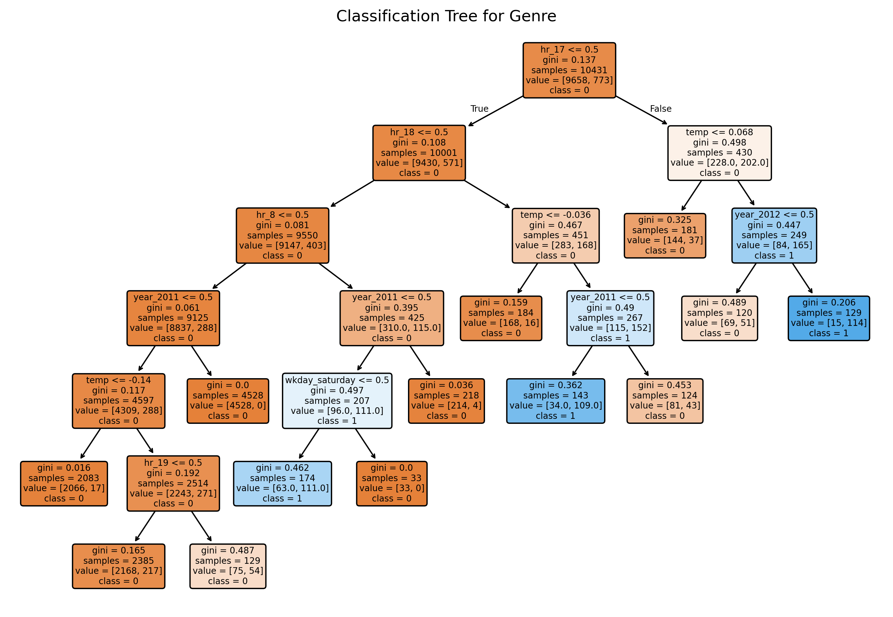
Fit a classification tree model with: - At least 200 samples to consider splitting a node. - The minimum reduction of 0.0005 in impurity required for a split to occur. - Limits the tree to 6 levels.

# In scikit-learn, we can use min_impurity_decrease=0.0005 for a similar effect.
tree_model = DecisionTreeClassifier(max_depth = 6, min_impurity_decrease=0.0005, min_samples_split=200, random_state=42)
# Fit the model using all predictors (all columns except 'medv')
tree_model.fit(X_train, y_train)


# Predict on training and test sets
y_train_pred = tree_model.predict(X_train)
y_test_pred = tree_model.predict(X_test)

# Plot the decision tree
plt.figure(figsize=(12, 8), dpi = 300)
plot_tree(tree_model, feature_names=X_train.columns, class_names= [str(cls) for cls in tree_model.classes_], filled=True, rounded=True)
plt.title("Classification Tree for Genre")
plt.show()

Question 12

Fit the following random forest regression model

\[ \begin{align} \text{cnt} =\ F\Big(&\beta_{\text{intercept}}\\ &+ \beta_{\text{temp}} \, \text{temp}_{i} + \beta_{\text{hum}} \, \text{hum}_{i} + \beta_{\text{windspeed}} \, \text{windspeed}_{i} \nonumber \\ &+ \beta_{\text{year\_2012}} \, \text{year\_2012}_{i}\\ &+ \beta_{\text{month\_2}} \, \text{month\_2}_{i} + \beta_{\text{month\_3}} \, \text{month\_3}_{i} + \beta_{\text{month\_4}} \, \text{month\_4}_{i} \nonumber \\ &+ \beta_{\text{month\_5}} \, \text{month\_5}_{i} + \beta_{\text{month\_6}} \, \text{month\_6}_{i} + \beta_{\text{month\_7}} \, \text{month\_7}_{i} + \beta_{\text{month\_8}} \, \text{month\_8}_{i} \nonumber \\ &+ \beta_{\text{month\_9}} \, \text{month\_9}_{i} + \beta_{\text{month\_10}} \, \text{month\_10}_{i} + \beta_{\text{month\_11}} \, \text{month\_11}_{i} + \beta_{\text{month\_12}} \, \text{month\_12}_{i} \nonumber \\ &+ \beta_{\text{hr\_1}} \, \text{hr\_1}_{i} + \beta_{\text{hr\_2}} \, \text{hr\_2}_{i} + \beta_{\text{hr\_3}} \, \text{hr\_3}_{i} + \beta_{\text{hr\_4}} \, \text{hr\_4}_{i} \nonumber \\ &+ \beta_{\text{hr\_5}} \, \text{hr\_5}_{i} + \beta_{\text{hr\_6}} \, \text{hr\_6}_{i} + \beta_{\text{hr\_7}} \, \text{hr\_7}_{i} + \beta_{\text{hr\_8}} \, \text{hr\_8}_{i} \nonumber \\ &+ \beta_{\text{hr\_9}} \, \text{hr\_9}_{i} + \beta_{\text{hr\_10}} \, \text{hr\_10}_{i} + \beta_{\text{hr\_11}} \, \text{hr\_11}_{i} + \beta_{\text{hr\_12}} \, \text{hr\_12}_{i} \nonumber \\ &+ \beta_{\text{hr\_13}} \, \text{hr\_13}_{i} + \beta_{\text{hr\_14}} \, \text{hr\_14}_{i} + \beta_{\text{hr\_15}} \, \text{hr\_15}_{i} + \beta_{\text{hr\_16}} \, \text{hr\_16}_{i} \nonumber \\ &+ \beta_{\text{hr\_17}} \, \text{hr\_17}_{i} + \beta_{\text{hr\_18}} \, \text{hr\_18}_{i} + \beta_{\text{hr\_19}} \, \text{hr\_19}_{i} + \beta_{\text{hr\_20}} \, \text{hr\_20}_{i} \nonumber \\ &+ \beta_{\text{hr\_21}} \, \text{hr\_21}_{i} + \beta_{\text{hr\_22}} \, \text{hr\_22}_{i} + \beta_{\text{hr\_23}} \, \text{hr\_23}_{i} \nonumber \\ &+ \beta_{\text{wkday\_monday}} \, \text{wkday\_monday}_{i} + \beta_{\text{wkday\_tuesday}} \, \text{wkday\_tuesday}_{i} + \beta_{\text{wkday\_wednesday}} \, \text{wkday\_wednesday}_{i} \nonumber \\ &+ \beta_{\text{wkday\_thursday}} \, \text{wkday\_thursday}_{i} + \beta_{\text{wkday\_friday}} \, \text{wkday\_friday}_{i} + \beta_{\text{wkday\_saturday}} \, \text{wkday\_saturday}_{i} \nonumber \\ &+ \beta_{\text{holiday\_1}} \, \text{holiday\_1}_{i} \nonumber \\ &+ \beta_{\text{seasons\_summer}} \, \text{seasons\_summer}_{i} + \beta_{\text{seasons\_fall}} \, \text{seasons\_fall}_{i} + \beta_{\text{seasons\_winter}} \, \text{seasons\_winter}_{i} \nonumber \\ &+ \beta_{\text{weather\_cond\_Light\_Snow\_or\_Light\_Rain}} \, \text{weather\_cond\_Light\_Snow\_or\_Light\_Rain}_{i}\nonumber \\ &+ \beta_{\text{weather\_cond\_Mist\_or\_Cloudy}} \, \text{weather\_cond\_Mist\_or\_Cloudy}_{i}\Big) \end{align} \]

with the following parameter setting:

• 19 predictors are allowed to consider when looking for the best split at each node in each tree
• 500 trees in the forest
• Useing out-of-bag samples to estimate error

# Build the Random Forest model
# max_features=13 means that at each split the algorithm randomly considers 13 predictors.
rf = RandomForestRegressor(max_features=19,  # Use 19 features at each split
                           n_estimators=500,  # Number of trees in the forest
                           random_state=42,
                           oob_score=True)    # Use out-of-bag samples to estimate error
rf.fit(X_train, y_train)


# Print the model details
print("Random Forest Model:")
print(rf)

# Output the model details (feature importances, OOB score, etc.)
print("Out-of-bag score:", rf.oob_score_)  # A rough estimate of generalization error


# Generate predictions on training and testing sets
y_train_pred = rf.predict(X_train)
y_test_pred = rf.predict(X_test)

# Calculate Mean Squared Errors (MSE) for both sets
train_mse = mean_squared_error(y_train, y_train_pred)
test_mse = mean_squared_error(y_test, y_test_pred)
print("Train MSE:", train_mse)
print("Test MSE:", test_mse)

# Optional: Plot predicted vs. observed values for test data
# plt.figure(figsize=(8,6), dpi=300)
# plt.scatter(y_test, y_test_pred, alpha=0.7)
# plt.plot([min(y_test), max(y_test)], [min(y_test), max(y_test)], 'r--')
# plt.xlabel("Observed medv")
# plt.ylabel("Predicted medv")
# plt.title("Random Forest: Observed vs. Predicted Values")
# plt.show()

Random Forest Model:
RandomForestRegressor(max_features=30, n_estimators=500, oob_score=True,
                      random_state=42)
Out-of-bag score: 0.7179654724578944
Train MSE: 0.002611945163455086
Test MSE: 0.021199175809935203

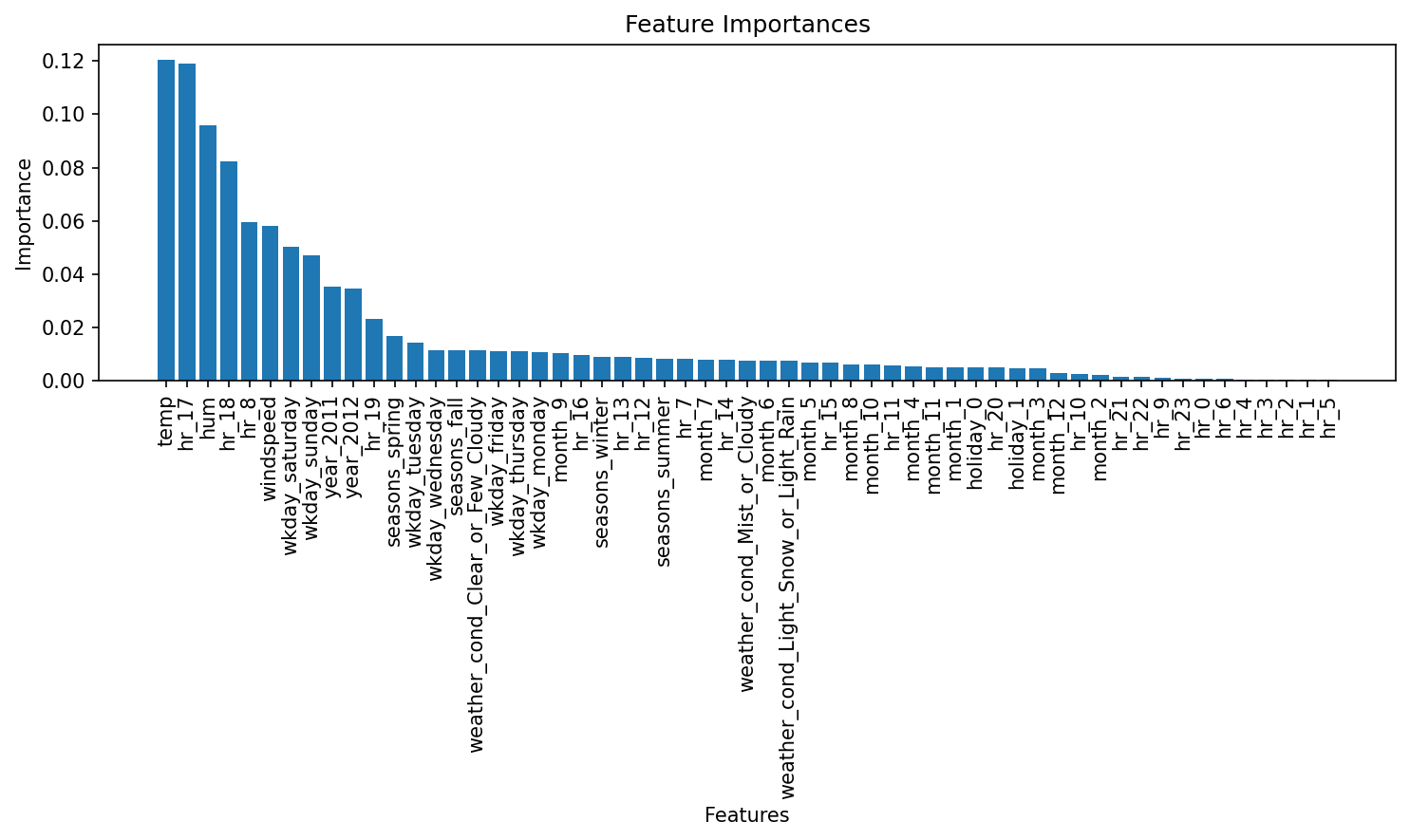
# Get feature importances from the model (equivalent to importance(bag.boston) in R)
importances = rf.feature_importances_
feature_names = X_train.columns

print("Feature Importances:")
for name, imp in zip(feature_names, importances):
    print(f"{name}: {imp:.4f}")

# Plot the feature importances, similar to varImpPlot(bag.boston) in R
# Sort the features by importance for a nicer plot.
indices = np.argsort(importances)[::-1]

plt.figure(figsize=(10, 6), dpi=150)
plt.title("Feature Importances")
plt.bar(range(len(feature_names)), importances[indices], align='center')
plt.xticks(range(len(feature_names)), feature_names[indices], rotation=90)
plt.xlabel("Features")
plt.ylabel("Importance")
plt.tight_layout()
plt.show()

Feature Importances:
temp: 0.1204
hum: 0.0960
windspeed: 0.0580
year_2011: 0.0351
year_2012: 0.0344
month_1: 0.0049
month_2: 0.0022
month_3: 0.0045
month_4: 0.0052
month_5: 0.0067
month_6: 0.0074
month_7: 0.0076
month_8: 0.0059
month_9: 0.0101
month_10: 0.0059
month_11: 0.0050
month_12: 0.0027
hr_0: 0.0005
hr_1: 0.0003
hr_2: 0.0003
hr_3: 0.0004
hr_4: 0.0004
hr_5: 0.0002
hr_6: 0.0004
hr_7: 0.0080
hr_8: 0.0595
hr_9: 0.0010
hr_10: 0.0024
hr_11: 0.0055
hr_12: 0.0085
hr_13: 0.0089
hr_14: 0.0076
hr_15: 0.0065
hr_16: 0.0094
hr_17: 0.1192
hr_18: 0.0823
hr_19: 0.0230
hr_20: 0.0048
hr_21: 0.0015
hr_22: 0.0012
hr_23: 0.0006
wkday_sunday: 0.0470
wkday_monday: 0.0105
wkday_tuesday: 0.0143
wkday_wednesday: 0.0113
wkday_thursday: 0.0108
wkday_friday: 0.0109
wkday_saturday: 0.0501
holiday_0: 0.0048
holiday_1: 0.0047
seasons_spring: 0.0166
seasons_summer: 0.0081
seasons_fall: 0.0112
seasons_winter: 0.0090
weather_cond_Clear_or_Few_Cloudy: 0.0112
weather_cond_Light_Snow_or_Light_Rain: 0.0072
weather_cond_Mist_or_Cloudy: 0.0076

Question 13

Fit the following gradient boosting regression model

\[ \begin{align} \text{cnt} =\ F\Big(&\beta_{\text{intercept}}\\ &+ \beta_{\text{temp}} \, \text{temp}_{i} + \beta_{\text{hum}} \, \text{hum}_{i} + \beta_{\text{windspeed}} \, \text{windspeed}_{i} \nonumber \\ &+ \beta_{\text{year\_2012}} \, \text{year\_2012}_{i}\\ &+ \beta_{\text{month\_2}} \, \text{month\_2}_{i} + \beta_{\text{month\_3}} \, \text{month\_3}_{i} + \beta_{\text{month\_4}} \, \text{month\_4}_{i} \nonumber \\ &+ \beta_{\text{month\_5}} \, \text{month\_5}_{i} + \beta_{\text{month\_6}} \, \text{month\_6}_{i} + \beta_{\text{month\_7}} \, \text{month\_7}_{i} + \beta_{\text{month\_8}} \, \text{month\_8}_{i} \nonumber \\ &+ \beta_{\text{month\_9}} \, \text{month\_9}_{i} + \beta_{\text{month\_10}} \, \text{month\_10}_{i} + \beta_{\text{month\_11}} \, \text{month\_11}_{i} + \beta_{\text{month\_12}} \, \text{month\_12}_{i} \nonumber \\ &+ \beta_{\text{hr\_1}} \, \text{hr\_1}_{i} + \beta_{\text{hr\_2}} \, \text{hr\_2}_{i} + \beta_{\text{hr\_3}} \, \text{hr\_3}_{i} + \beta_{\text{hr\_4}} \, \text{hr\_4}_{i} \nonumber \\ &+ \beta_{\text{hr\_5}} \, \text{hr\_5}_{i} + \beta_{\text{hr\_6}} \, \text{hr\_6}_{i} + \beta_{\text{hr\_7}} \, \text{hr\_7}_{i} + \beta_{\text{hr\_8}} \, \text{hr\_8}_{i} \nonumber \\ &+ \beta_{\text{hr\_9}} \, \text{hr\_9}_{i} + \beta_{\text{hr\_10}} \, \text{hr\_10}_{i} + \beta_{\text{hr\_11}} \, \text{hr\_11}_{i} + \beta_{\text{hr\_12}} \, \text{hr\_12}_{i} \nonumber \\ &+ \beta_{\text{hr\_13}} \, \text{hr\_13}_{i} + \beta_{\text{hr\_14}} \, \text{hr\_14}_{i} + \beta_{\text{hr\_15}} \, \text{hr\_15}_{i} + \beta_{\text{hr\_16}} \, \text{hr\_16}_{i} \nonumber \\ &+ \beta_{\text{hr\_17}} \, \text{hr\_17}_{i} + \beta_{\text{hr\_18}} \, \text{hr\_18}_{i} + \beta_{\text{hr\_19}} \, \text{hr\_19}_{i} + \beta_{\text{hr\_20}} \, \text{hr\_20}_{i} \nonumber \\ &+ \beta_{\text{hr\_21}} \, \text{hr\_21}_{i} + \beta_{\text{hr\_22}} \, \text{hr\_22}_{i} + \beta_{\text{hr\_23}} \, \text{hr\_23}_{i} \nonumber \\ &+ \beta_{\text{wkday\_monday}} \, \text{wkday\_monday}_{i} + \beta_{\text{wkday\_tuesday}} \, \text{wkday\_tuesday}_{i} + \beta_{\text{wkday\_wednesday}} \, \text{wkday\_wednesday}_{i} \nonumber \\ &+ \beta_{\text{wkday\_thursday}} \, \text{wkday\_thursday}_{i} + \beta_{\text{wkday\_friday}} \, \text{wkday\_friday}_{i} + \beta_{\text{wkday\_saturday}} \, \text{wkday\_saturday}_{i} \nonumber \\ &+ \beta_{\text{holiday\_1}} \, \text{holiday\_1}_{i} \nonumber \\ &+ \beta_{\text{seasons\_summer}} \, \text{seasons\_summer}_{i} + \beta_{\text{seasons\_fall}} \, \text{seasons\_fall}_{i} + \beta_{\text{seasons\_winter}} \, \text{seasons\_winter}_{i} \nonumber \\ &+ \beta_{\text{weather\_cond\_Light\_Snow\_or\_Light\_Rain}} \, \text{weather\_cond\_Light\_Snow\_or\_Light\_Rain}_{i}\nonumber \\ &+ \beta_{\text{weather\_cond\_Mist\_or\_Cloudy}} \, \text{weather\_cond\_Mist\_or\_Cloudy}_{i}\Big) \end{align} \]

with the following grid of hyperparameters

param_grid = {
    "n_estimators": list(range(20, 201, 20)),  # nrounds: 20, 40, ..., 200
    "learning_rate": [0.025, 0.05, 0.1, 0.3],    # eta
    "gamma": [0],                               # gamma
    "max_depth": [1, 2, 3, 4],
    "colsample_bytree": [1],
    "min_child_weight": [1],
    "subsample": [1]
}

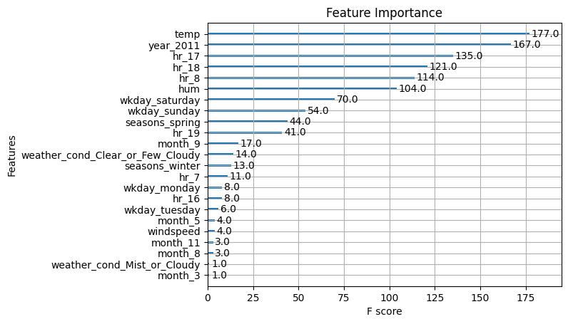
# Define the grid of hyperparameters
param_grid = {
    "n_estimators": list(range(20, 201, 20)),  # nrounds: 20, 40, ..., 200
    "learning_rate": [0.025, 0.05, 0.1, 0.3],    # eta
    "gamma": [0],                               # gamma
    "max_depth": [1, 2, 3, 4],
    "colsample_bytree": [1],
    "min_child_weight": [1],
    "subsample": [1]
}

# Initialize the XGBRegressor with the regression objective and fixed random state for reproducibility
xgb_reg = XGBRegressor(objective="reg:squarederror", random_state=1937, verbosity=1)

# Set up GridSearchCV with 10-fold cross-validation; scoring is negative MSE
grid_search = GridSearchCV(
    estimator=xgb_reg,
    param_grid=param_grid,
    scoring="neg_mean_squared_error",
    cv=5,
    verbose=1  # Adjust verbosity as needed
)

# Fit the grid search
grid_search.fit(X_train, y_train)

# Train the final model using the best parameters (grid_search.best_estimator_ is already refit on entire data)
final_model = grid_search.best_estimator_

# Plot variable importance using XGBoost's plot_importance function
plt.figure(figsize=(10, 8))
plot_importance(final_model)
plt.title("Feature Importance")
plt.show()

# Calculate MSE on the training data
y_pred_train = final_model.predict(X_train)
train_mse = mean_squared_error(y_train, y_pred_train)
print("Train MSE:", train_mse)

# Calculate MSE on the test data
y_pred = final_model.predict(X_test)
test_mse = mean_squared_error(y_test, y_pred)
print("Test MSE:", test_mse)

# Print the best parameters found by GridSearchCV
best_params = grid_search.best_params_
print("Best parameters:", best_params)

Fitting 10 folds for each of 160 candidates, totalling 1600 fits

<Figure size 1000x800 with 0 Axes>

Train MSE: 0.03805126994848251
Test MSE: 0.038990434259176254
Best parameters: {'colsample_bytree': 1, 'gamma': 0, 'learning_rate': 0.025, 'max_depth': 3, 'min_child_weight': 1, 'n_estimators': 160, 'subsample': 1}

Question 14

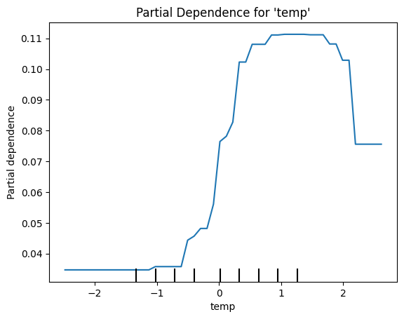
Using the gradient boosting model, generate a partial dependence plot for the predictor temp, illustrating its average effect on the predicted outcome.

# Plot partial dependence for the predictor 'off'
feature_names = X_train.columns.tolist()
off_index = feature_names.index("temp")
PartialDependenceDisplay.from_estimator(final_model, X_train, features=[off_index],
                                        feature_names=feature_names, kind="average")
plt.title("Partial Dependence for 'temp'")
plt.show()

Question 15

Below is the summary table of the model fit from Question 1 in Section 1:

• Interpret the beta estimates for the following predictors:
  1. temp
  2. hum
  3. year_2012

Question 16

Below is the summary table of the marginal effects at the mean from Question 4 in Section 1:

• Interpret the estimate for the temp predictor:

Question 17

Below is the confusion matrix from Question 6 in Section 1:

• Interpret the following metrics:
  • Accuracy
  • Precision
  • Recall

Question 18

Suppose you’re the manager of DC Bike. When there’s a high number of bike requests (cnt > 500), your team becomes overloaded, and you must pay $100/hr in overtime to handle the excess demand. Alternatively, you can avoid the risk of overtime by hiring an extra driver ahead of time at a fixed cost of $50/hr.

However, overload doesn’t happen every hour—sometimes it does, sometimes it doesn’t. Let’s say the probability of an overload happening in a given hour is p, and the probability of no overload is 1 - p.

You want to decide whether it’s worth hiring an extra driver ahead of time or taking the chance and only paying overtime if needed. To make this decision, compare (1) the expected cost of not hiring no extra driver with (2) the cost of hiring an extra driver, which is $50/hr.

Expected cost is the weighted average cost you’d expect in the long run, if you made the same decision many times under the same conditions.

It is calculated as:

(Expected Cost) = (Cost of Outcome 1 × Probability of Outcome 1) + (Cost of Outcome 2 × Probability of Outcome 2) + …

Option 1: No Extra Driver

• If no overload:
  Cost = $0, Probability = 1 - p

• If overload:
  Cost = $100, Probability = p

Option 2: Hire an Extra Driver

• You always pay $50, regardless of whether overload happens or not.

At what value of p (probability of over_load = 1) is it cheaper on average to hire the extra driver?

Question 19

Below is the classification tree from Question 11 in Section 2:

• Interpret the following two leaf nodes and explain the decision rules that lead to them:
  • Leaf Node 1
    • gini = 0.0
    • samples = 4258
    • value = [4258, 0]
    • class = 0
  • Leaf Node 2
    • gini = 0.206
    • samples = 129
    • value = [15, 114]
    • class = 1

Question 20

Compare and interpret the predictive performance and potential overfitting of the Random Forest and Gradient Boosting models based on the following results obtained in Questions 12 and 13:

• Random Forest
  • Training MSE: 0.0026
  • Test MSE: 0.0212
• Gradient Boosting
  • Training MSE: 0.0381
  • Test MSE: 0.0390

In your answer, evaluate how well each model performs on unseen data and explain whether there is evidence of overfitting in either model.

Question 21

Consider the following linear regression models:

• Model 1 \[ \text{yield}_{i} = \beta_0 + \beta_{\text{fertilizer}}\text{fertilizer}_i + \epsilon_i \]

• Model 2 \[ \text{yield}_{i} = \beta_0 + \beta_{\text{fertilizer}}\text{fertilizer}_i + \beta_{\text{height}}\text{height}_i + \epsilon_i \]

• Model 3 \[ \text{yield}_{i} = \beta_0 + \beta_{\text{fertilizer}}\text{fertilizer}_i + \beta_{\text{height}}\text{height}_i + \beta_{\text{soil\_quality}}\text{soil\_quality}_i + \epsilon_i \]

• fertilizer: Indicator equal to 1 if the plot received fertilizer, 0 otherwise.

• height: Plant height (in centimeters), which itself depends on fertilizer and soil quality.

• soil_quality: Underlying soil fertility (standardized index), unobserved by the researcher.

• yield: Crop yield (in bushels) for each plot.

It is known that the true value of beta coefficients are as follows:

• \(\beta_{\text{fertilizer}} = 10\); \(\beta_{\text{height}} = 0.5\); \(\beta_{\text{soil\_quality}} = 7.5\)

RMSE_1	RMSE_2	RMSE_3
1232.779	88.69368	57.42429

Q21a

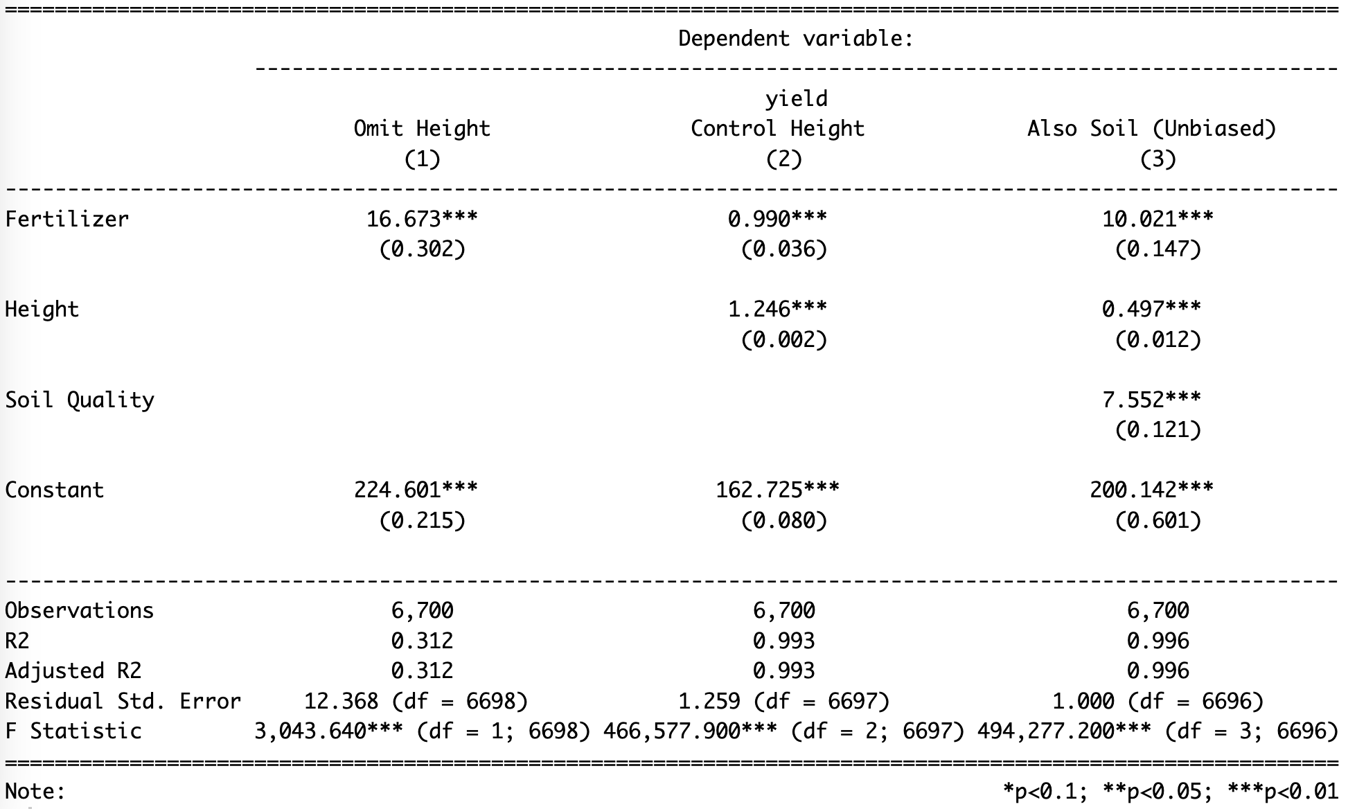
• Calculate the magnitude of bias in the estimated \(\text{fertilizer}\) coefficient for Model 1 and for Model 2.

Q21b

1. Why does including \(\text{height}\) (Model 2) worsen the bias in \(\hat\beta_{\text{fertilizer}}\) and decrease the test‑set RMSE?
2. Given what regression finds about the coefficient, explain how partialling out \(\text{height}\) change the “independent” part of \(\text{fertilizer}\)?
3. When does adding a predictor make things worse, and when does it help?

• Under what circumstances will including an extra predictor increase both coefficient bias and RMSE?
• Under what circumstances will it instead reduce bias and improve predictive accuracy?