Lecture 9
K-fold Cross-Validation; Regularized Regression
March 26, 2025
\(K\)-fold Cross-Validation
K-fold Cross-Validation

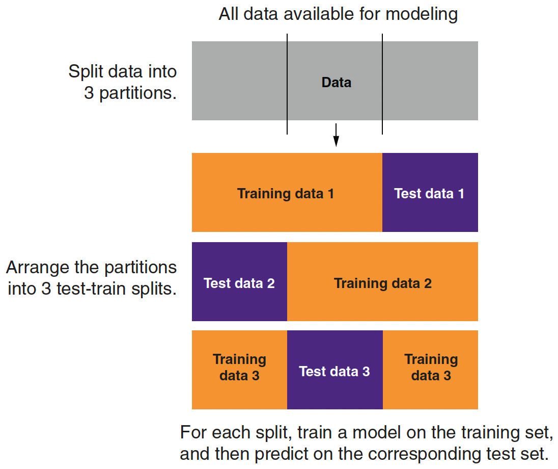
Partitioning Data for 3-fold Cross-Validation
- A single train–test split uses each subset only once—either for training or for evaluation.
- K‑fold cross-validation divides the training data into K equal parts (folds).
- For each fold \(k=1, \dots, K\):
- Step 1: Train the model on \(K‑1\) folds.
- Step 2: Evaluate the model on the held‑out fold.
- For each fold \(k=1, \dots, K\):
- The average error (e.g., deviance) across folds provides a robust estimate of model performance.
Training, Validation, and Test Datasets
Training Data:
The portion of data used to fit the model.
Within this set, k‑fold cross-validation is applied.Validation Data:
Temporary splits within the training set during cross-validation, used to tune hyperparameters and assess performance.Test Data:
A held-out dataset that is never used during model tuning.
Provides an unbiased evaluation of the final model’s performance.Workflow:
- Split: Divide the dataset into training and test sets.
- Cross-Validate: Apply k‑fold CV on the training set for model tuning and selection.
- Evaluate: Use the test set for final performance assessment.
- Split: Divide the dataset into training and test sets.
Regularization
Regularization
Regularized regression can resolve the following problems:
- Quasi-separation in logistic regression
- Multicolinearity in linear regression
- e.g., Variables \(\texttt{age}\) and \(\texttt{years_of_workforce}\) in linear regression of \(\texttt{income}\).
- Overfitting
The above situations usually happen when the model is too complex (e.g., has large or many beta variables).
We will discuss three regularized regression methods:
- Lasso or LASSO (least absolute shrinkage and selection operator) (L1)
- Ridge (L2)
- Elastic net
What is Linear Regression Doing?
- Regular linear regression tries to find the beta parameters \(\beta_0, \beta_1, \beta_2, \,\cdots\, \beta_{p}\) such that
\[ f(x_i) = b_0 + b_1 x_{1,i} + b_2 x_{2,i} + \,\cdots\, + b_p x_{p,i} \] is as close as possible to \(y_i\) for all the training data by minimizing the sum of the squared error (SSE) between \(y\) and \(f(x)\) with observations \(i = 1, \cdots, N\), where the SSE is
\[ (y_1 - f(x_1))^2 + (y_2 - f(x_2))^2 + \,\cdots\, + (y_N - f(x_N))^2 \]
What is Lasso Regression Doing?
- Lasso regression tries to find the beta parameters \(\beta_0, \beta_1, \beta_2, \,\cdots\, \beta_{p}\) and \(\alpha\) such that
\[ f(x_i) = b_0 + b_1 x_{1,i} + b_2 x_{2,i} + \,\cdots\, + b_p x_{p,i} \] is as close as possible to \(y_i\) for all the training data by minimizing the sum of the squared error (SSE) plus the sum of the absolute value of the beta parameters multiplied by the alpha parameter:
\[ \begin{align} &(y_1 - f(x_1))^2 + (y_2 - f(x_2))^2 + \,\cdots\, + (y_N - f(x_N))^2 \\ &+ \alpha \times(| \beta_1 | + |\beta_2 | + \,\cdots\, + |\beta_{p}|) \end{align} \] - When \(\alpha = 0\), this reduces to regular linear regression.
What is Lasso Regression Doing?
When variables are nearly collinear, lasso regression tends to drive one or more of them to zero.
In the regression of \(\text{income}\), lasso regression might give zero credit to one of the two variables, \(\texttt{age}\) and \(\texttt{years_of_workforce}\).
For this reason, lasso regression is often used as a form of model/variable selection.
What is Ridge Regression Doing?
- Ridge regression tries to find the beta parameters \(\beta_0, \beta_1, \beta_2, \,\cdots\, \beta_{p}\) and \(\alpha\) such that
\[ f(x_i) = b_0 + b_1 x_{1,i} + b_2 x_{2,i} + \,\cdots\, + b_p x_{p,i} \] is as close as possible to \(y_i\) for all the training data by minimizing the sum of the squared error (SSE) plus the sum of the squared beta parameters multiplied by the alpha parameter:
\[ \begin{align} &(y_1 - f(x_1))^2 + (y_2 - f(x_2))^2 + \,\cdots\, + (y_N - f(x_N))^2 \\ &+ \alpha \times (\beta_1^2 + \beta_2^2 + \,\cdots\, + \beta_{p}^2) \end{align} \] - When \(\alpha = 0\), this reduces to regular linear regression.
What is Ridge Regression Doing?
- When variables are nearly collinear, ridge regression tends to average the collinear variables together.
- You can think of this as “ridge regression shares the credit.”
- Imagine that being one year older/one year longer in the workforce increases \(\texttt{income}\) in the training data.
- In this situation, ridge regression might give a half credit to each variable of \(\texttt{age}\) and \(\texttt{years_of_workforce}\), which adds up to the appropriate effect.
What is Elastic Net Regression Doing?
- Elastic net regression tries to find the beta parameters \(\beta_0, \beta_1, \beta_2, \,\cdots\, \beta_{p}\) and \(\lambda\) (L1 parameter) such that
\[ f(x_i) = b_0 + b_1 x_{1,i} + b_2 x_{2,i} + \,\cdots\, + b_p x_{p,i} \] is as close as possible to \(y_i\) for all the training data by minimizing the sum of the squared error (SSE) plus a linear combination of the ridge and the lasso penalties with the \(\lambda\) parameter:
\[ \begin{align} &(y_1 - f(x_1))^2 + (y_2 - f(x_2))^2 + \,\cdots\, + (y_N - f(x_N))^2 \\ &+ \lambda \times(| \beta_1 | + |\beta_2 | + \,\cdots\, + |\beta_{p}|)\\ &+ (1-\lambda) \times(\beta_1^2 + \beta_2^2 + \,\cdots\, + \beta_{p}^2) \end{align} \]
where \(0 \leq \lambda \leq 1\).
Choosing Between Lasso, Ridge, and Elastic Net
- In some situations, such as when you have a very large number of variables, many of which are correlated to each other, the lasso may be preferred.
- In other situations, like quasi-separability, the ridge solution may be preferred.
- When you are not sure which is the best approach, you can combine the two by using elastic net regression.
- Different values of \(\lambda\) between 0 and 1 give different trade-offs between sharing the credit among correlated variables, and only keeping a subset of them.
Intuition on Different Penalties

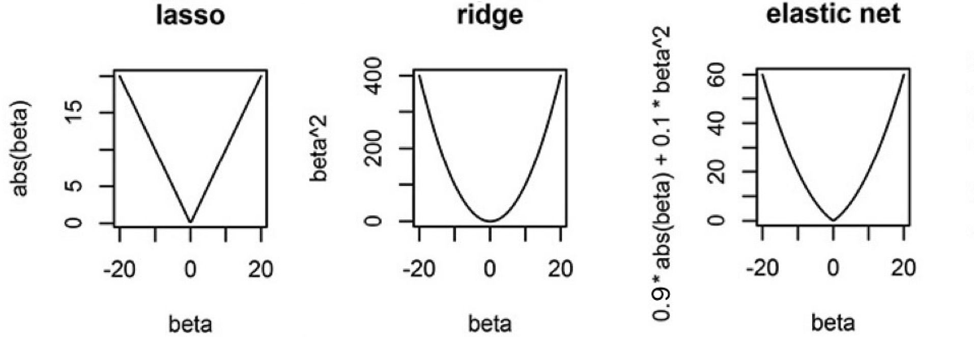
- Lasso (L1) Penalty (\(|\beta|\)):
- Each unit increase in \(\beta\) adds a constant penalty, regardless of \(\beta\) ’s size.
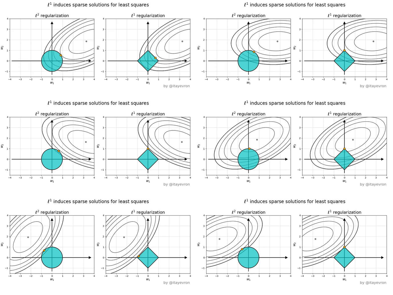
- Drives some coefficients exactly to zero, acting as a predictor selection mechanism.
- Ridge (L2) Penalty (\(\beta^2\)):
- Gently penalizes small-to-moderate deviations from zero, but penalty increases quickly for large \(\beta\).
- Shrinks coefficients but does not set them exactly to zero.
Intuition on Different Penalties

- Lasso induces corner solutions!
Regularization Affects the Interpretation of Beta
- No Need to Omit a Reference Category:
- In standard regression, one dummy is typically omitted to avoid perfect multicollinearity.
- Even though including all dummies creates perfect collinearity with an intercept, regularization resolves this by penalizing the beta parameters.
- In regularized regression, the penalty term handles multicollinearity by shrinking all coefficients, so you can include all dummy variables.
- Each coefficient then represents the deviation from a shared baseline (an implicit average effect).
- In standard regression, one dummy is typically omitted to avoid perfect multicollinearity.
- Interpretation:
- With this approach, we interpret a dummy’s beta as how much that category’s association with the outcome, without worrying about the reference level (intercept).
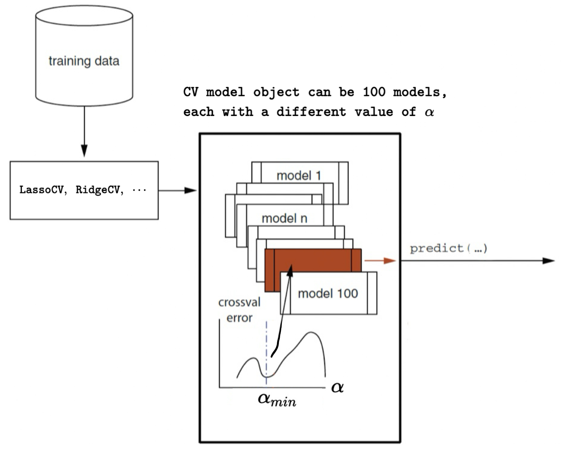
Regularized Regression with Cross-Validation with scikit-learn

- \(\alpha_{min}\): the \(\alpha\) for the model with the minimum cross-validation (CV) error
Regularized Logistic Regression with scikit-learn
Python Libraries and Modules for Regularization
Here are the required libraries and modules for logistic regression with regularization:
import pandas as pd
import numpy as np
import matplotlib.pyplot as plt
import seaborn as sns

from sklearn.model_selection import train_test_split
from sklearn.linear_model import LogisticRegression, LogisticRegressionCV
from sklearn.metrics import (confusion_matrix, accuracy_score, precision_score,
                             recall_score, roc_curve, roc_auc_score)
Data Preparation with train_test_split() and pd.get_dummies()
cars = pd.read_csv('https://bcdanl.github.io/data/car-data.csv')

# Split into train and test (70% train, 30% test)
# Using a fixed random state for reproducibility (seed = 24351)
cars_train, cars_test = train_test_split(cars, test_size=0.3, random_state=24351)

# Define predictors: all columns except "rating" and "fail"
predictors = [col for col in cars.columns if col not in ['rating', 'fail']]

# One-hot encode categorical predictors.
X_train = pd.get_dummies(cars_train[predictors])
X_test = pd.get_dummies(cars_test[predictors])
# Ensure that the test set has the same dummy columns as the training set
X_test = X_test.reindex(columns=X_train.columns)

# Outcome variable
y_train = cars_train['fail'].astype(int)
y_test = cars_test['fail'].astype(int)
Lasso - LogisticRegressionCV(penalty='l1', solver='saga')
lasso_cv = LogisticRegressionCV(Cs=100, cv=5,
  penalty='l1', solver='saga', max_iter=1000, scoring='neg_log_loss')
lasso_cv.fit(X_train, y_train)Cs=100: Tries 100 different values of regularization strength (1/C)cv=5: Uses 5-fold cross-validationpenalty='l1': Applies L1 regularization (Lasso)solver='saga'Supports L1 regularizationmax_iter=1000: Sets the maximum number of iterations for solver to convergescoring='neg_log_loss': Uses deviance as the CV performance metric.fit(X_train, y_train): Fits the model; Selects the best \(\alpha = \frac{1}{C}\).
Lasso Logistic Regression (L1) - Full Code
# Note: solver='saga' supports L1 regularization.
lasso_cv = LogisticRegressionCV(
    Cs=100, cv=5, penalty='l1', solver='saga', max_iter=1000, scoring='neg_log_loss'
)
lasso_cv.fit(X_train, y_train)

intercept = float(lasso_cv.intercept_)
coef_lasso = pd.DataFrame({
    'predictor': list(X_train.columns),
    'coefficient': list(lasso_cv.coef_[0])
})

print("Lasso Regression Coefficients:")
print(coef_lasso)

# Force an order for the y-axis (using the feature names as they appear in coef_lasso)
order = coef_lasso['predictor'].tolist()

plt.figure(figsize=(8,6))
ax = sns.pointplot(x="coefficient", y="predictor", data=coef_lasso, order=order, join=False)
plt.title("Coefficients of Lasso Logistic Regression Model")
plt.xlabel("Coefficient value")
plt.ylabel("Predictor")

# Draw horizontal lines from 0 to each coefficient.
for _, row in coef_lasso.iterrows():
    # Get the y-axis position from the order list.
    y_pos = order.index(row['predictor'])
    plt.hlines(y=y_pos, xmin=0, xmax=row['coefficient'], color='gray', linestyle='--')

# Draw a vertical line at 0.
plt.axvline(0, color='black', linestyle='--')

plt.show()

# Prediction and evaluation for lasso model
y_pred_prob_lasso = lasso_cv.predict_proba(X_test)[:, 1]
y_pred_lasso = (y_pred_prob_lasso > 0.5).astype(int)
ctab_lasso = confusion_matrix(y_test, y_pred_lasso)
accuracy_lasso = accuracy_score(y_test, y_pred_lasso)
precision_lasso = precision_score(y_test, y_pred_lasso)
recall_lasso = recall_score(y_test, y_pred_lasso)
auc_lasso = roc_auc_score(y_test, y_pred_prob_lasso)

print("Confusion Matrix (Lasso):\n", ctab_lasso)
print("Lasso Accuracy:", accuracy_lasso)
print("Lasso Precision:", precision_lasso)
print("Lasso Recall:", recall_lasso)


# Plot ROC Curve
fpr, tpr, thresholds = roc_curve(y_test, y_pred_prob_lasso)
plt.figure(figsize=(8,6))
plt.plot(fpr, tpr, label=f'Lasso (AUC = {auc_ridge:.2f})')
plt.plot([0, 1], [0, 1], 'k--', label='Random Guess')
plt.xlabel('False Positive Rate')
plt.ylabel('True Positive Rate')
plt.title('ROC Curve for Lasso Logistic Regression Model')
plt.legend(loc='best')
plt.show()
Ridge (L2) - LogisticRegressionCV(penalty='l2')
ridge_cv = LogisticRegressionCV(Cs=100, cv=5,
  penalty='l2', solver='lbfgs', max_iter=1000, scoring='neg_log_loss'
)
ridge_cv.fit(X_train, y_train)penalty='l2': Applies L2 regularization (Ridge)solver='lbfgs'Supports L2 regularization (optional)
Ridge Logistic Regression (L2) - Full Code
# LogisticRegressionCV automatically selects the best regularization strength.
ridge_cv = LogisticRegressionCV(
    Cs=100, cv=5, penalty='l2', solver='lbfgs', max_iter=1000, scoring='neg_log_loss'
)
ridge_cv.fit(X_train, y_train)

print("Ridge Regression - Best C (inverse of regularization strength):", ridge_cv.C_[0])
intercept = float(ridge_cv.intercept_)
coef_ridge = pd.DataFrame({
    'predictor': list(X_train.columns),
    'coefficient': list(ridge_cv.coef_[0])
})
print("Ridge Regression Coefficients:")
print(coef_ridge)

# Force an order for the y-axis (using the feature names as they appear in coef_ridge)
order = coef_ridge['predictor'].tolist()

plt.figure(figsize=(8,6))
ax = sns.pointplot(x="coefficient", y="predictor", data=coef_ridge, order=order, join=False)
plt.title("Coefficients of Ridge Logistic Regression Model")
plt.xlabel("Coefficient value")
plt.ylabel("Predictor")

# Draw horizontal lines from 0 to each coefficient.
for _, row in coef_ridge.iterrows():
    # Get the y-axis position from the order list.
    y_pos = order.index(row['predictor'])
    plt.hlines(y=y_pos, xmin=0, xmax=row['coefficient'], color='gray', linestyle='--')

# Draw a vertical line at 0.
plt.axvline(0, color='black', linestyle='--')
plt.show()

# Prediction and evaluation for ridge model
y_pred_prob_ridge = ridge_cv.predict_proba(X_test)[:, 1]
y_pred_ridge = (y_pred_prob_ridge > 0.5).astype(int)
ctab_ridge = confusion_matrix(y_test, y_pred_ridge)
accuracy_ridge = accuracy_score(y_test, y_pred_ridge)
precision_ridge = precision_score(y_test, y_pred_ridge)
recall_ridge = recall_score(y_test, y_pred_ridge)
auc_ridge = roc_auc_score(y_test, y_pred_prob_ridge)

print("Confusion Matrix (Ridge):\n", ctab_ridge)
print("Ridge Accuracy:", accuracy_ridge)
print("Ridge Precision:", precision_ridge)
print("Ridge Recall:", recall_ridge)


# Plot ROC Curve
fpr, tpr, thresholds = roc_curve(y_test, y_pred_prob_ridge)
plt.figure(figsize=(8,6))
plt.plot(fpr, tpr, label=f'Ridge (AUC = {auc_ridge:.2f})')
plt.plot([0, 1], [0, 1], 'k--', label='Random Guess')
plt.xlabel('False Positive Rate')
plt.ylabel('True Positive Rate')
plt.title('ROC Curve for Ridge Logistic Regression Model')
plt.legend(loc='best')
plt.show()
Elastic Net - LogisticRegressionCV(penalty='l2')
enet_cv = LogisticRegressionCV(
    Cs=10, cv=5, penalty='elasticnet', solver='saga',
    l1_ratios=[0.5, 0.7, 0.9], max_iter=1000, scoring='neg_log_loss'
)
enet_cv.fit(X_train, y_train)Cs=10: Tries 10 different values of regularization strength (1/C)cv=5: Uses 5-fold cross-validationpenalty='elasticnet': Applies Elastic Net regularizationl1_ratios = [0.5, 0.7, 0.9]In this model, we try 0.5, 0.7, 0.9l1_ratio = 1→ Lassol1_ratio = 0→ Ridge
Elastic Net Logistic Regression - Full Code
# LogisticRegressionCV supports elastic net penalty with solver 'saga'.
# l1_ratio specifies the mix between L1 and L2 (0 = ridge, 1 = lasso).
enet_cv = LogisticRegressionCV(
    Cs=10, cv=5, penalty='elasticnet', solver='saga',
    l1_ratios=[0.5, 0.7, 0.9], max_iter=1000, scoring='neg_log_loss'
)
enet_cv.fit(X_train, y_train)

print("Elastic Net Regression - Best C:", enet_cv.C_[0])
print("Elastic Net Regression - Best l1 ratio:", enet_cv.l1_ratio_[0])

intercept = float(enet_cv.intercept_)
coef_enet = pd.DataFrame({
    'predictor': list(X_train.columns),
    'coefficient': list(enet_cv.coef_[0])
})
print("Elastic Net Regression Coefficients:")
print(coef_enet)


# Force an order for the y-axis (using the feature names as they appear in coef_lasso)
order = coef_enet['predictor'].tolist()

plt.figure(figsize=(8,6))
ax = sns.pointplot(x="coefficient", y="predictor", data=coef_enet, order=order, join=False)
plt.title("Coefficients of Elastic Net Logistic Regression Model")
plt.xlabel("Coefficient value")
plt.ylabel("Predictor")

# Draw horizontal lines from 0 to each coefficient.
for _, row in coef_enet.iterrows():
    # Get the y-axis position from the order list.
    y_pos = order.index(row['predictor'])
    plt.hlines(y=y_pos, xmin=0, xmax=row['coefficient'], color='gray', linestyle='--')

# Draw a vertical line at 0.
plt.axvline(0, color='black', linestyle='--')

plt.show()

# Prediction and evaluation for elastic net model
y_pred_prob_enet = enet_cv.predict_proba(X_test)[:, 1]
y_pred_enet = (y_pred_prob_enet > 0.5).astype(int)
ctab_enet = confusion_matrix(y_test, y_pred_enet)
accuracy_enet = accuracy_score(y_test, y_pred_enet)
precision_enet = precision_score(y_test, y_pred_enet)
recall_enet = recall_score(y_test, y_pred_enet)

print("Confusion Matrix (Elastic Net):\n", ctab_enet)
print("Elastic Net Accuracy:", accuracy_enet)
print("Elastic Net Precision:", precision_enet)
print("Elastic Net Recall:", recall_enet)
Regularized Linear Regression with scikit-learn
Lasso Linear Regression
- The browser dataset contains web browsing logs for 10,000 households.
- The browser dataset include a year’s worth of their browser logs for the 1,000 most heavily trafficked websites
- Each browser in the sample spent at least $1 online in the same year.
\[ \log(\text{spend}_{i}) = \beta_0 + \beta_1 X_{1,i} +\,\cdots\,+ \beta_{1000} X_{1000,i} + \epsilon_i \] - \(\text{spend}_{i}\): household \(i\)’s amount of dollars spent on online shopping - \(X_{p, i}\) household \(i\)’s percentage of visiting the \(p\) website
Lasso Linear Regression - Libraries and Modules
from google.colab import data_table
data_table.enable_dataframe_formatter()  # Enabling an interactive DataFrame display
import numpy as np
import pandas as pd
import matplotlib.pyplot as plt
import seaborn as sns

from sklearn.preprocessing import scale   # zero mean & one s.d.
from sklearn.linear_model import LassoCV, lasso_path
from sklearn.model_selection import train_test_split
from sklearn.metrics import mean_squared_error
Lasso Linear Regression - Data Prep
df = pd.read_csv("https://bcdanl.github.io/data/browser-online-shopping.zip")

X = df.drop('spend', axis = 1)
y = df['spend']

# Train-test split
X_train, X_test, y_train, y_test = train_test_split(X, y, test_size=0.2, random_state=42)

X_train_np = X_train.values
X_test_np = X_test.values
y_train_np = y_train.values
y_test_np = y_test.values
Lasso Linear Regression - Fitting the Model
Lasso Linear Regression - Results
# Best alpha
print("LassoCV - Best alpha:", lasso_cv.alpha_)

# Create a DataFrame including the intercept and the coefficients:
coef_lasso = pd.DataFrame({
    'predictor': list(X_train.columns),
    'coefficient':  list(lasso_cv.coef_),
    'exp_coefficient': np.exp(  list(lasso_cv.coef_) )
})

# Evaluate
y_pred_lasso = lasso_cv.predict(X_test)
mse_lasso = mean_squared_error(y_test, y_pred_lasso)
print("LassoCV - MSE:", mse_lasso)

coef_lasso = coef_lasso.query('coefficient != 0')
coef_lasso.shape[0]
coef_lasso.sort_values('coefficient', ascending = False)
Lasso Path - CV Errors as as a Function of Alpha
# Compute the mean and standard deviation of the CV errors for each alpha.
mean_cv_errors = np.mean(lasso_cv.mse_path_, axis=1)
std_cv_errors = np.std(lasso_cv.mse_path_, axis=1)

plt.figure(figsize=(8, 6))
plt.errorbar(lasso_cv.alphas_, mean_cv_errors, yerr=std_cv_errors, marker='o', linestyle='-', capsize=5)
plt.xscale('log')
plt.xlabel('Alpha')
plt.ylabel('Mean CV Error (MSE)')
plt.title('Cross-Validation Error vs. Alpha')
plt.axvline(x=lasso_cv.alpha_, color='red', linestyle='--', label='Best alpha')
plt.legend()
plt.show()
Lasso Path - Beta Estimates as a Function of Alpha
# Compute the lasso path. Note: we use np.log(y_train) because that's what you used in LassoCV.
alphas, coefs, _ = lasso_path(X_train, np.log(y_train), alphas=lasso_cv.alphas_, max_iter=100000)

plt.figure(figsize=(8, 6))
# Iterate over each predictor and plot its coefficient path.
for i, col in enumerate(X_train.columns):
    plt.plot(alphas, coefs[i, :], label=col)

plt.xscale('log')
plt.xlabel('Alpha')
plt.ylabel('Coefficient value')
plt.title('Lasso Coefficient Paths')
plt.axvline(x=lasso_cv.alpha_, color='red', linestyle='--', label='Best alpha')
plt.show()
Lasso Path - The Number of Nonzero Betas as a Function of Alpha
# Compute the coefficient path over the alpha grid that LassoCV used
alphas, coefs, _ = lasso_path(X_train, np.log(y_train),
                              alphas=lasso_cv.alphas_,
                              max_iter=100000)

# Count nonzero coefficients for each alpha (coefs shape: (n_features, n_alphas))
nonzero_counts = np.sum(coefs != 0, axis=0)

# Plot the number of nonzero coefficients versus alpha
plt.figure(figsize=(8,6))
plt.plot(alphas, nonzero_counts, marker='o', linestyle='-')
plt.xscale('log')
plt.xlabel('Alpha')
plt.ylabel('Number of nonzero coefficients')
plt.title('Nonzero Coefficients vs. Alpha')
#plt.gca().invert_xaxis()  # Lower alphas (less regularization) on the right
plt.axvline(x=lasso_cv.alpha_, color='red', linestyle='--', label='Best alpha')
plt.legend()
plt.show()
Hockey Player Performance via Regularized Logistic Regression
Background and Motivation
- The player “plus-minus” (PM) is a common hockey performance metric.
- The classic PM is a function of goals scored while that player is on the ice:
- the number of goals for his team minus the number against.
- The limits of this approach are obvious: there is no accounting for teammates or opponents.
- In hockey, where players tend to be grouped together on “lines” and coaches will “line match” against opponents, a player’s PM can be artificially inflated or deflated by the play of his opponents and peers.
Data
The data comprise of play-by-play NHL game data for regular and playoff games during 11 seasons of 2002-2003 through 2013-2014.
There were p = 2,439 players involved in n = 69,449 goals.
The data contains information that indicates seasons, home & away teams, team configuration such as 5 on 4 powerplay, and which players are on & off the ice when a goal is made, etc.
Unfortunately, Python
scikit-learnis not optimized to handle all season’s data.- What we can do with Python
scikit-learnis handling one season each. - I highly recommend R’s
glmnetfor regression with cross-validation.
- What we can do with Python
Data
homegoal: an indicator (0 or 1) for the home team scoringplayer_name: entries for who was on the ice for each goalteam: indicators for each teamconfig: Special teams info. E.g.,S5v4is a 5 on 4 powerplay- The value of
config,team, andplayer_nameare:- 1 if it is for the home-team
- -1 for the away team
- 0 otherwise
Model
- Consider constructing a binary response for every goal, equal to 1 for home-team goals and 0 for away-team goals:
\[ \begin{align} \log\left(\frac{\text{Prob}(\text{home-goal}_{i})}{\text{Prob}(\text{away-goal}_{i})}\right) &= \beta_0 + \sum_{j=1}^{J} \beta_{\text{team}_{j}}\text{team}_{j, i} + \sum_{k=1}^{K} \beta_{\text{config}_{k}}\text{config}_{k, i} \\ &\qquad + \sum_{m=1}^{M} \beta_{\text{home-player}_{m}}\text{home-player}_{m, i}\\ &\qquad - \sum_{n=1}^{N} \beta_{\text{away-player}_{n}}\text{away-player}_{n, i} \end{align} \]
Home-ice Advantage
Player’s Impact
Traditional Plus‑Minus vs. Expected Plus‑Minus
- Traditional Plus‑Minus (PM)
- Definition: Sum of on-ice contributions; +1 for a goal scored for the player’s team and -1 for a goal against.
- Limitations: Can be noisy due to team context, limited ice time, or random variation.
- Expected Plus‑Minus (ppm)
- Definition: A model-based estimate of a player’s impact.
- Calculation:
- Convert a player’s effect (\(\beta\)) to a probability: \(p = \frac{e^{\beta}}{1 + e^{\beta}}\)
- Compute expected PM as: \(\text{ppm} = ng \times p − ng \times (1−p )\)
- \(ng\): the total number of goals the player was on the ice.
- Benefits: Smooths out noise and adjusts for context.
Traditional Plus‑Minus vs. Expected Plus‑Minus
- Observed vs. Modeled:
- PM is a raw, observed measure.
- Expected PM leverages model estimates to predict performance.
- PM is a raw, observed measure.
- Variability:
- PM may fluctuate due to external factors.
- Expected PM attempts to isolate a player’s true impact.
- PM may fluctuate due to external factors.
- Applications:
- Expected PM can help identify under- or over-performing players and guide strategic decisions.
Scaling?
- We do not want to standardize variables here.
- The penalty with standardization is \(\alpha \times SD(X_{player})\)
- Players with small SD are those who play little (almost all zeros).
- Players with large SD are those who play a lot.
- Standardization would up-weight the influence of players who rarely play relative to those who have a lot of ice time.
- Re-do everything with
Omitted Variable Bias
Omitted Variable Bias
Omitted variable bias (OVB): bias in the model because of omitting an important predictor that is correlated with existing predictor(s).
Let’s use an orange juice (OJ) example to demonstrate the OVB.
- OJ price elasticity estimates vary with models, whether or not taking into account
brandorad_status
- OJ price elasticity estimates vary with models, whether or not taking into account
Short- and Long- Regressions
OVB is the difference in beta estimates between short- and long-form regressions.
Short regression: The regression model with less predictors
\[ \begin{align} \log(\text{sales}_i) = \beta_0 + \beta_1\log(\text{price}_i) + \epsilon_i \end{align} \]
- Long regression: The regression model that adds additional predictor(s) to the short one.
\[ \begin{align} \log(\text{sales}_i) =& \beta_0 + \beta_{1}\log(\text{price}_i) \\ &+ \beta_{2}\text{minute.maid}_i + \beta_{3}\text{tropicana}_i + \epsilon_i \end{align} \] - OVB for \(\beta_1\) is:
\[ \text{OVB} = \widehat{\beta_{1}^{short}} - \widehat{\beta_{1}^{long}} \]
OVB formula
Consider the following short- and long- regressions:
- Short: \(Y_i = \beta_0 + \beta_{1}^{short}X_1 + \epsilon_{short}\)
- Long: \(Y_i = \beta_0 + \beta_{1}^{long}X_1 +\beta_{2}X_2 + \epsilon_{long}\)
- Short: \(Y_i = \beta_0 + \beta_{1}^{short}X_1 + \epsilon_{short}\)
Error in short form can be represented as: \[ {\epsilon_{short}} = \beta_{2}X_2 + \epsilon_{long} \]
If variable \(X_1\) is correlated with \(X_2\), the following assumptions are violated in the short regression model:
- Errors are not correlated with predictors.
- Errors have a mean value of 0.
How does an OVB happen in regression?
- In the first stage, consider the relationship between
priceandbrand:
\[ \log(\text{price}) = \beta_0 + \beta_1\text{minute_maid} + \beta_2\text{tropicana} + \epsilon_{1st} \]
Then, calculate the residual: \[ \widehat{\epsilon_{1st}} = \log(\text{price}) - \widehat{\log(\text{price})} \]
The residual represents the log of OJ price after its correlation with brand has been removed!
In the second stage, regress \(\log(\text{sales})\) on residual \(\widehat{\epsilon_{1st}}\):
\[ \log(\text{sales}) = \beta_0 + \beta_1\widehat{\epsilon_{1st}} + \epsilon_{2nd} \]
Regression Sensitivity Analysis
Regression finds the coefficients on the part of each predictor that is independent from the other predictors.
What can we do to deal with OVB problems?
- Because we can never be sure whether a given set of controls is enough to eliminate OVB, it’s important to ask how sensitive regression results are to changes in the list of controls.

